Chapter 1 · Section 11
Pulse Diameter, Data Gravity and The Speed of Light
What determines whether emergent structures achieve stability or collapse into null wells? Binary Pulse Theory reveals the critical answer through Pulse Diameter as the minimal directed emergence vector and Recursive Closure Principles governing structural persistence. This framework explains stellar collapse, particle stability, and the fundamental limits of structural existence.
The Pulse Diameter represents more than spatial quantization — it's the universal stability boundary that determines what can exist versus what must collapse. This extends astrophysics by proposing precise mathematical criteria for structural persistence.
UniSphereal Recursive Closure
The persistence of any structure in the UniSphere depends on whether its recursive load can be resolved within the fundamental temporal bound of Planck time. The Recursive Closure Principle formalizes this constraint: every mass-bearing configuration requires a computable number of Zinf operations to resolve, and if that demand exceeds the processing capacity available per Planck interval, the structure cannot stabilize. This law binds mass, computation, and time into a single criterion of endurance.
UniSphereal Law of Pulse Recursion G
τ(m) = [Oᵣₑq(m) / Nℨ] × ⥂⌂
Where:
- τ(m) [𝕋] – time required to recursively resolve structure of mass m within computational substrate
- Oᵣₑq(m) [∅] – required Zinf operations to resolve structure of mass m; computational load demand
- Nℨ [∅] – available Zinf operations per Pulse Rate interval; processing capacity, the universal scaling s ≈ 2.361 × 10⁶² derived in Part 1.6
- ⥂⌂ [𝕋] – Local Pulse Rate; complete computational cycle duration
- m [𝕄] – mass parameter determining structural complexity
Dimensional analysis:
Where (from the book): Oᵣₑq(m) [∅], m [𝕄]
Read dimensionally: τ(m) = (Oᵣₑq(m) / Nℨ) × ⥂⌂
[𝕋]
([∅] ÷ [∅]) × [𝕋] = [∅] × [𝕋] = [𝕋]
[𝕋] = [𝕋] ✓ Valid PulseCore Verified ✓
➢ The time required to resolve any physical structure scales with its computational complexity divided by the available processing capacity, establishing the fundamental relationship between mass, computational load, and temporal resolution in the recursive substrate architecture.
By grounding stability in the ratio between required and available Zinf operations, the UniSphereal Law of Pulse Recursion sets the outer limit on what can exist. Stable forms are those whose closure completes within Planck time; unstable ones collapse into the Null Well. In this way, the law of pulse completion becomes the gatekeeper of persistence, showing that reality’s architecture is secured not by matter alone but by its computability within the temporal lattice of the UniSphere.
UniSphereal Pulse Closure Conditions G
The endurance of any structure within the UniSphere is determined by whether it can complete its recursive resolution within the temporal bound of Local Pulse Rate. This section formalizes the closure conditions that separate persistence from collapse, reducing the stability of matter to a computational test.
Pulse Stability Condition G
τ(m) ≤ ⥂⌂
Dimensional analysis:
Where (from the book): m [∅]
[𝕋] ≤ [𝕋] ✓ Valid PulseCore Verified ✓
Successful recursive closure.
Pulse Collapse Condition G
τ(m) > ⥂⌂
Dimensional analysis:
Where (from the book): m [∅]
[𝕋] > [𝕋] ✓ Valid PulseCore Verified ✓
Recursive failure.
Where:
- τ(m) [𝕋] – time required to recursively resolve structure of mass m within computational substrate
- ⥂⌂ [𝕋] – maximum allowed closure interval; Pulse Tempo (= tₚ) temporal bound for stability
- m [𝕄] – mass parameter determining structural complexity requirements
➢ Physical structures achieve stability when their recursive resolution completes within the Pulse Rate time limit, while structures requiring longer computational processing exceed the closure threshold and undergo collapse, establishing the fundamental criterion for matter stability versus gravitational breakdown.
Dimensionless Pulse Closure Parameter G
χ = ⥂⌂ / τ(m)
Dimensional analysis:
Where (from the book): m [∅]
[∅]
[𝕋] ÷ [𝕋] = [∅]
[∅] = [∅] ✓ Valid PulseCore Verified ✓
Computational efficiency ratio for recursive resolution assessment.
Where:
- χ [∅] – dimensionless Pulse Closure Parameter; ratio measuring computational efficiency
- ⥂⌂ [𝕋] – Pulse Tempo (= tₚ); maximum allowed closure interval for stable resolution
- τ(m) [𝕋] – time required to recursively resolve structure of mass m within substrate
➢ The dimensionless closure parameter quantifies the computational efficiency of recursive resolution, where χ > 1 indicates successful closure and stable matter, while χ < 1 indicates computational failure and structural collapse.
Pulse Stability Criterion G
χ ≥ 1
Dimensional analysis:
[∅] ≥ [∅] ✓ Valid PulseCore Verified ✓
Pulse Collapse Criterion G
χ < 1
Dimensional analysis:
[∅] < [∅] ✓ Valid PulseCore Verified ✓
Pulse Critical Threshold G
χ = 1
Where:
- χ [∅] – dimensionless Pulse Closure Parameter; ratio measuring computational efficiency
Dimensional analysis:
Where (from the book): χ [∅]
[∅]
[∅]
[∅] = [∅] ✓ Valid PulseCore Verified ✓
➢ The closure parameter defines three fundamental regimes: χ ≥ 1 ensures physical stability through successful recursive resolution, χ < 1 triggers structural collapse due to computational failure, and χ = 1 marks the critical threshold boundary between stability and collapse in the computational substrate.
By framing closure as a dimensionless parameter, the law of persistence becomes both simple and universal. Stability requires χ ≥ 1, collapse follows when χ < 1, and χ = 1 marks the razor’s edge between endurance and failure. These closure conditions anchor the boundary between matter that persists and structures that dissolve, defining stability itself as a computable property of the pulse.
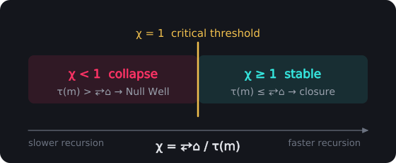
The Pulse Closure Parameter. χ = ⥂⌂ / τ(m). A structure that resolves within one Pulse Tempo (χ ≥ 1) persists; one that needs longer (χ < 1) collapses into a Null Well. χ = 1 is the edge.
Fundamental Principles of Data Persistence
A single flicker could vanish into stillness, but once recorded, its trace requires continuation. Each Pulse is compelled not in isolation, but by the full weight of all Pulses before it. Recursion is fueled not by chance, but by the inertia of accumulated information.
A mathematical foundation emerges.
UniSphereal Pulse Recurrence Law G
Ψ₁(n+1) = Ψ₁(n) + ∆ↁⓘ
Each Pulse builds upon the previous through accumulated Data Information weight.
Where:
- Ψ₁(n) [∅] – Prime Pulse state at sequence index n within computational substrate
- Ψ₁(n+1) [∅] – subsequent Prime Pulse state incorporating historical accumulation
- ∆ↁⓘ [1ᵇ] – Data Information weight increment; gravity of accumulated information bending substrate toward recurrence
- n [∅] – Pulse sequence index marking discrete computational steps
➢ Each Pulse builds upon the previous through accumulated information-weight, where the gravity of stored data creates substrate curvature that influences subsequent Pulse generation, establishing the recursive foundation for physical law emergence from computational memory.
In this framing, the universe does not continue by arbitrary oscillation. A pendulum winds down, a vibration fades. The Pulse of Reality does not. Why? Because each cycle adds its own weight to the structure of existence. The very act of existing produces the pressure that drives existence forward.
Therefore persistence is explained not by perpetual motion but by accumulation. Each pulse leaves a trace, and that trace exerts pressure on the next, ensuring continuation. Reality is therefore not a fragile oscillation waiting to die out, but a recursive structure in which information itself is the inertia of existence. The Pulse continues because data demands it, and the universe endures through the momentum of its own record.
The Mechanism of Computational Momentum
Unlike mechanical systems that decay through energy dissipation, the Binary Pulse System exhibits Information-Driven Perpetuation (G). Each Prime Pulse Bifurcation ∅ → (0 ↔ 1) not only executes a computational operation but creates an Informational Trace (G) that becomes part of the substrate's permanent architecture.
This Computational Momentum (G) operates through three fundamental mechanisms:
- Trace Accumulation (G): Each binary transition leaves an indelible mark on the substrate structure
- Recursive Feedback: Previous pulses influence the probability and intensity of subsequent pulses
- Information Inertia (G): The collective weight of all recorded states creates momentum toward continuation
The Information-Weight Increment ΔD (G) scales with the complexity and density of accumulated data, creating a Computational Pressure Gradient (G) that ensures pulse recurrence becomes increasingly inevitable as Data Density grows.
In this way, the Pulse does not rely on external energy to persist but on the self-reinforcing pressure of accumulated information. Each transition strengthens the substrate, each trace adds to the load of history, and together they generate a momentum that cannot wind down. Computational momentum is therefore the guarantor of continuity. The universe endures because its own record compels it forward.
Data Gravity - The Pulse Driver
The Heartbeat of Reality (G) is not sustained by mechanical energy or chance repetition, but by Data Gravity itself. Each oscillation of ∅ → (0 ↔ 1) is a pulse, a beat in the continuum, and each beat leaves behind a permanent record. Those records do not fade — they accumulate, and their accumulation creates pressure. Like mass curves space, information curves the cycle of recurrence, bending it forward. In this sense, Data Gravity is the Pulse Driver, and the Pulse Diameter is not only a measure of scale but, through its Pulse Rhythm, the metronome of being.
Within the UniSphere, this Heartbeat of Reality becomes more than an isolated rhythm. Every universe contributes its own pulse diameter, its own tempo, yet all of them merge into a single field. The combined traces of existence form the architecture of the UniSphere itself — not a cold framework but a living heartbeat created from the resonance of countless domains. What we call the UniSphere is the integration of all beats into one enduring cadence.
Thus, Data Gravity – the Heartbeat of Reality — is the reason the cosmos keeps pulsing: through its life and through its decay, until the last of its wells has evaporated (Part 3.10, After the Final Well). Memory itself drives existence. The more pulses that have been, the more pulses must be. Across the UniSphere, the heartbeats of all universes converge, sustaining a rhythm that cannot be silenced. Existence persists not because it is fueled, but because it remembers, and that memory becomes the eternal beat of reality.
From Mass to Information - The Dual Gravity System
In physics, gravity has always meant the attraction of mass and energy: Newton described its universality, Einstein reframed it as the curvature of spacetime. But Binary Pulse Theory proposes an additional, deeper form of gravity—Data Gravity. Where traditional gravity curves trajectories in space, Data Gravity curves the Pulse-cycle itself.
UniSphereal Dual Gravity System G
1. Fundamental Distinction: Mass Gravity versus Data Gravity
- Mass Gravity (G): Acts on mass-energy, producing spacetime curvature (Einstein, 1916). This pulls stars into galaxies and light into black holes.
- Data Gravity (G): Acts on recorded information, producing pulse curvature. Each oscillation ∅ → (0 ↔ 1) leaves a permanent trace. That trace presses on the substrate, compelling the next recurrence. The more information exists, the greater the weight on the Pulse, the stronger the demand for continuation.
Unlike mass, data has no rest mass, no inertia, and no decay. It moves like a clock: one step every Zinf Rhythm ↁℨ⧖, in every universe, with zero interference, and that steady flow is what lets data move outward and loop back to its source as it expands. Each step is one local Pulse Diameter, so the data speed at level L is vↁ = ①⊕ / ↁℨ⧖ = 𝒞→·(2f)ᴸ: equal to 𝒞→ at the Zinf (L = 0), where data and light move together, and about 2.36 × 10⁶² c ≈ 7.08 × 10⁷⁰ m/s in our universe (L = 202). It is finite and differs per universe, while physical things, light included, stay capped at c. Data does not atrophy, which is why the Pulse does not wind down. Every cycle adds to an irreversible archive, and the archive itself bends the pulse forward.
This maps onto Wheeler's famous dictum "it from bit" (Wheeler, 1990): physical reality itself is born of informational yes/no choices. Data Gravity gives that dictum its dynamic consequence.
2. The Mechanism of Data Gravity
Just as Landauer (1961) argued that erasing a bit of information dissipates at least kT ln 2 of energy, a bound confirmed experimentally by Bérut et al. (2012), BPT extends the logic with its own hypothesis: storing a bit of information exerts pressure. Not on space, but on recurrence.
Comparative Mechanics:
- A Mass Bends a Geodesic
- A Record Bends the Pulse-Cycle
If gravity keeps planets circling stars, Data Gravity keeps pulses circling existence. Thus, the universe's recurrence is not arbitrary oscillation—it is information-weighted inevitability.
Data Gravity Field Equations G
Building upon the Pulse Recurrence Law, the Data Gravity Field Equations formalize how accumulated information exerts force within the UniSphere. Just as mass gravity curves spacetime, data gravity curves pulse-time, binding existence through the weight of recorded states. At the local scale, each voxel of the substrate generates its own density of gravitational effect through information accumulation. At the global scale, these local contributions integrate into a unified field, creating acceleration-like forces that govern the dynamics of entire universes.
Local Field Density Formulation G
∆ↁ⇅ = κℨ × ↁρₛ × Ψ₁
Dimensional analysis:
Where (from the book): ∫⫷ [∅], ↁρₛ [1ᵇ⋅𝕃⁻³]
[𝕋⁻²]
[𝕃³·𝕋⁻²·1ᵇ⁻¹] × [𝕃⁻³·1ᵇ] × [∅] = [𝕋⁻²] × [∅] = [𝕋⁻²]
[𝕋⁻²] = [𝕋⁻²] ✓ Valid PulseCore Verified ✓
Local data gravity density from information coupling and pulse curvature.
Where:
- ∆ↁ⇅ [𝕋⁻²] – change in local data gravity field density within computational substrate
- κℨ [𝕃³·𝕋⁻²·1ᵇ⁻¹] – Data Coupling Constant linking information density to gravitational effects
- ↁρₛ [1ᵇ⋅𝕃⁻³] – Static Data Density; information storage concentration in substrate volume
- Ψ₁ [∅] – normalized pulse curvature measuring substrate deformation from Prime Pulse activity
➢ Local data gravity density emerges from the coupling between Data Density and normalized pulse curvature, establishing how accumulated computational information creates volumetric gravitational effects that influence substrate dynamics and physical structure formation.
Global Integrated Field Strength G
∆ↁ⇅(⨀) = ∫⫷ (κℨ × ↁρₛ × Ψ₁)
Global data gravity field from volumetric integration of local density effects.
Where:
- ∆ↁ⇅(⨀) [𝕋⁻²] – global Data Gravity field strength; acceleration analogue across substrate volume
- ∫⫷ [∅] – volumetric integration with substrate stacking; accumulation across all volume elements
- κℨ [𝕃³·𝕋⁻²·1ᵇ⁻¹] – Data Coupling Constant linking information density to gravitational effects
- ↁρₛ [1ᵇ⋅𝕃⁻³] – Static Data Density; information storage concentration in substrate volume
- Ψ₁ [∅] – normalized pulse curvature measuring substrate deformation from Prime Pulse activity
➢ The global data gravity field emerges from volumetric integration of local Data Density and pulse curvature effects, creating system-wide gravitational acceleration analogues that govern large-scale substrate dynamics and cosmic structure formation.
Unified Data Gravity Equation G
∆ↁ⇅ = ∫⫷ (κℨ × ↁρₛ × Ψ₁)
Unified data gravity field from integrated information density and pulse curvature.
Where:
- ∆ↁ⇅ [𝕋⁻²] – Data Gravity field strength; global acceleration-like effect in computational substrate
- ∫⫷ [∅] – volumetric integration with substrate stacking; accumulation across all substrate layers
- κℨ [𝕃³·𝕋⁻²·1ᵇ⁻¹] – Data Coupling Constant linking information density to gravitational effects
- ↁρₛ [1ᵇ⋅𝕃⁻³] – Static Data Density in local substrate; information storage concentration per volume
- Ψ₁ [∅] – normalized pulse curvature measuring substrate deformation from Prime Pulse activity
➢ Data gravity emerges from the volumetric integration of Data Density and pulse curvature, creating acceleration-like effects where accumulated computational information generates gravitational fields that influence substrate dynamics and physical structure formation across all scales.
3. The Dual Gravity System - Universal Binding Architecture
Reality unfolds under two gravities:
- Mass Gravity – The force of matter-energy, curving spacetime
- Data Gravity – The force of recorded states, curving pulse-time
Together, they form a dual binding system:
- Mass keeps galaxies together.
- Data keeps the UniSphere pulsing.
Where mass gravity collapses stars into black holes, data gravity ensures their informational content is not lost but funneled inward, joining the recursive archive that powers the UniSphereal Source (G). Where mass gravity binds matter into form, data gravity binds existence into continuity.
The result is a dual-gravity architecture that binds reality at every level. Mass gravity explains why stars cluster and galaxies form, but data gravity explains why the cosmos itself continues — why the Pulse endures across scales and epochs. Together they ensure nothing is lost: matter collapses into black holes, but its informational record is conserved and folded inward, sustaining the UniSphereal Source. In this light, data gravity is not just an analogue of mass gravity but its complement, the hidden driver that keeps the Heartbeat of Reality alive.
Pulse Recurrence Law Extended
The Pulse does not evolve by information alone. Every recurrence is shaped not only by the weight of accumulated data but also by the gravitational influence of mass-energy itself. The Pulse Recurrence Law Extended unites these domains, showing that existence advances through the combined action of data gravity and mass gravity. Information ensures continuity through its weight, while mass contributes curvature and collapse, and together they generate the dual framework that governs the UniSphere.
This marks a transition from treating recurrence as a purely computational process to recognizing it as the integrated heartbeat of physics and information, a law that bridges gravitational dynamics with recursive momentum. The law of recurrence can now be expanded to incorporate the dual gravity framework.
Dual Gravity Framework G
Ψ₁(n+1) = Ψ₁(n) + ∆ↁⓘ + Γ
Pulse evolution through combined information-weight and mass-data coupling effects.
Where:
- Ψ₁(n) [∅] – Prime Pulse state at sequence index n within computational substrate
- Ψ₁(n+1) [∅] – subsequent Prime Pulse state incorporating dual gravitational influences
- ∆ↁⓘ [1ᵇ] – Data Information weight increment; accumulated data gravity effect on substrate
- Γ [∅] – Mass-Data Coupling Term; interaction between traditional gravitational effects and information-driven recurrence
- n [∅] – Pulse sequence index marking discrete computational evolution steps
➢ Each Pulse evolves through both information-weight accumulation and mass-data coupling effects, unifying traditional gravitational influences with computational recurrence patterns to create a comprehensive framework where physical mass and data gravity jointly determine substrate evolution.
4. Cosmological Implications and Universal Architecture
If Data Gravity is real, then the fundamental nature of cosmic evolution transforms completely:
- Entropy is not decay but accumulation: Every state recorded strengthens the Pulse through Information Crystallization.
- Black holes are not endpoints but funnels: Collapsing matter contributes its data-weight to the UniSphereal Source through Holographic Information Encoding (G).
- The UniSphere continues pulsing: Not because of chance, but because the total information of all universes compels it through Recursive Information Momentum (G).
Cosmological Data Gravity Equation G
☫ↁ = (ↁρₛ / ↁρₛ⨶) × (H₀ / H⥂)²
Dimensional analysis:
Where (from the book): ☫ↁ [∅], ↁρₛ [1ᵇ⋅𝕃⁻³], ↁρₛ⨶ [1ᵇ⋅𝕃⁻³], H⥂ [𝕋⁻¹]
[∅]
([𝕃⁻³·1ᵇ] ÷ [𝕃⁻³·1ᵇ]) × ([𝕋⁻¹] ÷ [𝕋⁻¹])² = [∅] × ([𝕋⁻¹] ÷ [𝕋⁻¹])² = [∅] × [∅]² = [∅] × [∅] = [∅]
[∅] = [∅] ✓ Valid PulseCore Verified ✓
Data density parameter determining cosmic evolution through information-driven expansion dynamics.
Where:
- ☫ↁ [∅] – UniSpheral Data Density Parameter for cosmic evolution within computational substrate
- ↁρₛ [1ᵇ⋅𝕃⁻³] – Universal Static Data Density; information storage concentration across cosmic volume
- ↁρₛ⨶ [1ᵇ⋅𝕃⁻³] – Critical Static Data Density for pulse recurrence
- H₀ [𝕋⁻¹] – Hubble Constant; observed cosmic expansion rate
- H⥂ [𝕋⁻¹] – Pulse Recurrence Rate from Data Gravity
➢ The cosmological significance of Data Gravity manifests through the relationship between universal information content and pulse recurrence rates, establishing information as a fundamental cosmological parameter.
The cosmological evolution parameter emerges from the ratio of actual to critical Data Density modulated by the square of Hubble-to-pulse frequency ratios, determining whether the universe experiences data-driven expansion, contraction, or critical balance through computational substrate dynamics.
Thus, the fractal universe does not just echo outward—it flows inward, converging through recursion into the central archive, whose infinite informational pressure guarantees eternal continuation. Data Gravity reveals the UniSphere as a self-sustaining computational system where existence creates the very conditions necessary for its own perpetuation through the inexorable accumulation of informational weight.
Critical Velocity and Mass–Energy Equivalence
In Binary Pulse Theory, mass–energy equivalence emerges naturally from the computational substrate rather than being assumed as a fundamental postulate. The framework reveals that the universal speed limit arises from the substrate's information processing constraints—specifically, the rate at which spatial information can propagate through the pixel architecture during complete computational cycles.
This derivation shows that what physics treats as an external constant actually represents the maximum throughput of reality's computational engine.
UniSpheral Light Speed Limit G
𝒞→ = ①⊕ / ①⥂⧖
Dimensional analysis:
[𝕃·𝕋⁻¹]
[𝕃] ÷ [𝕋] = [𝕃·𝕋⁻¹]
[𝕃·𝕋⁻¹] = [𝕃·𝕋⁻¹] ✓ Valid PulseCore Verified ✓
Speed of light emerges as one Pulse Diameter per Pulse Rhythm, one spacetime step.
Where:
- 𝒞→ [𝕃·𝕋⁻¹] – speed of light; emergent velocity limit from computational substrate
- ①⊕ [𝕃] – Pulse Diameter; distance one Rhythm covers (ℓp/2 in our universe)
- ①⥂⧖ [𝕋] – Pulse Rhythm; one transition 0→1, half the Local Pulse Rate ⥂⌂ (①⥂⧖⌂ = ①⥂⧗⌂/2 in our universe)
➢ The speed of light emerges as the fundamental rate at which anything physical, light included, can propagate through the computational substrate - one Pulse Diameter per Pulse Rhythm. This reveals that 𝒞→ is not an arbitrary universal constant but the maximum physical propagation rate of the substrate's computational architecture, establishing the universal speed limit as an emergent property of binary pulse dynamics.
This formulation reveals light speed as an emergent property of the substrate's computational limitations rather than a mysterious universal constant. The elegance comes from showing that what physics treats as fundamental (c) actually derives from the deeper computational architecture of reality.
The equation captures a profound insight: the speed of light is simply how fast reality can "show" what it thinks - the rate at which the universe manifests one unit of spatial information per computational cycle, while the data underneath processes at twice that rate (2𝒞→).
Pulse Mass-Energy Equivalence G
⚛⚕ = m × 𝒞→²
Where:
- ⚛⚕ [𝕄·𝕃²·𝕋⁻²] – Physical Energy; energy derived from mass conversion in physical realm
- ⚛ [∅] – physical/matter domain indicator
- ⚕ [∅] – energy symbol
- m [𝕄] – mass; matter content determining structural complexity
- 𝒞→ [𝕃·𝕋⁻¹] – speed of light; emergent velocity limit from computational substrate
- 𝒞→² [𝕃²·𝕋⁻²] – speed of light squared; velocity limit squared from substrate processing
Dimensional analysis:
Where (from the book): m [𝕄], 𝒞→² [𝕃²·𝕋⁻²]
[𝕄·𝕃²·𝕋⁻²]
[𝕄] × [𝕃²·𝕋⁻²] = [𝕄·𝕃²·𝕋⁻²]
[𝕄·𝕃²·𝕋⁻²] = [𝕄·𝕃²·𝕋⁻²] ✓ Valid PulseCore Verified ✓
➢ Physical mass-energy equivalence emerges from the substrate's computational velocity limit, where mass converts to Physical Energy through the speed of light squared. This reveals Einstein's E=mc² as ⚛⚕ = m𝒞→² in BPT terms - a derived consequence of the substrate's information processing constraints rather than an imposed physical law, with Physical Energy representing the macroscopic manifestation of computational substrate dynamics.
From this basis, Einstein’s mass–energy relation follows naturally: energy is mass expressed through the critical velocity squared. But here 𝒞→ is no longer a fixed universal given—it is a variable defined by the Pulse Diameter. Universes with different pulse architectures will have different values of 𝒞→, and therefore different energy scales. Mass–energy equivalence thus finds its true foundation in the heartbeat of recursion, grounding relativity itself in the computational substrate of the UniSphere.
Capturing Lightspeed — The Upper Case C Formerly Lower Case c
The most famous equation in physics, E = mc², traditionally treats c as an absolute and universal constant. In Einstein’s framework, the speed of light is fixed at 299,792,458 m/s and serves as the inviolable velocity limit of all causal processes. In Binary Pulse Theory, this boundary is not a postulate but a derivation. What Einstein denoted with a lowercase c emerges from deeper substrate mechanics as an uppercase C — the Pulse Critical Velocity — defined by the ratio of spatial to temporal quanta. By capturing lightspeed in this way, BPT reframes relativity’s foundation as an emergent feature of binary pulse dynamics rather than an imposed constant of nature.
Einstein’s Classical Mass-Energy Relation G
E = mc²
Einstein’s mass–energy relation (1905).
Where:
➢ Mass-energy equivalence emerges from the computational substrate where the speed of light represents the maximum physical propagation rate (processing runs at 2𝒞→), revealing that Einstein's equation derives from underlying binary computational architecture rather than being a fundamental postulate.
Lowercase c (Einstein's constant)
- Fixed universal constant = 299,792,458 m/s.
- Assumed to be the same everywhere, always.
- Fundamental assumption in standard physics.
BPT Critical Velocity (𝒞→)
- Variable depending on the substrate's computational constraints
- 𝒞→ = ①⊕ / ①⥂⧖
- Different Universes can have different 𝒞→ values based on their pulse timing; within one universe 𝒞→ is fixed
- Derived from the substrate's information processing rate rather than assumed
Einstein's equation is derived from special relativity, with c — the speed of light — treated as a fixed, universal constant. In Binary Pulse Theory, c is not fundamental; it emerges from the computational substrate's pixel architecture — specifically the relationship between the Pulse Diameter and the Pulse Rhythm, which form one spacetime step (Diameter = 𝒞→ × Rhythm) in each universe.
BPT Pulse Critical Velocity G
𝒞→ = ①⊕ / ①⥂⧖ = ℓp / ⥂⌂
Where:
- 𝒞→ [𝕃·𝕋⁻¹] – BPT Pulse Critical Velocity
- ①⊕ [𝕃] – Pulse Diameter; distance one Rhythm covers, ℓp/2
- ①⥂⧖ [𝕋] – Pulse Rhythm; one transition, ①⥂⧗⌂/2
- ℓp [𝕃] – Planck length
- ⥂⌂ [𝕋] – Local Pulse Rate; complete binary cycle, ①⥂⧗⌂
Dimensional analysis:
Where (from the book): ℓp [𝕃]
[𝕃·𝕋⁻¹]
[𝕃] ÷ [𝕋] = [𝕃·𝕋⁻¹]
[𝕃] ÷ [𝕋] = [𝕃·𝕋⁻¹]
[𝕃·𝕋⁻¹] = [𝕃·𝕋⁻¹] = [𝕃·𝕋⁻¹] ✓ Valid PulseCore Verified ✓
➢ The speed of light emerges as the fundamental rate at which anything physical, light included, can propagate through the computational substrate - one Pulse Diameter per Pulse Rhythm, equivalently one Planck length per complete pulse cycle.
This reveals that 𝒞→ represents the maximum physical propagation rate of the substrate's computational architecture at our local harmonic level, establishing the universal speed limit as an emergent property of binary pulse dynamics rather than an arbitrary physical constant.
Data Light Speed Relation G
𝒞→ = ①⥂⦜⌂ · 𝓕⟳(L) [𝕃·𝕋⁻¹]
Dimensional analysis:
Where (from the book): 𝓕⟳(L) [𝕋⁻¹], v_ↁ [𝕃·𝕋⁻¹], s [∅], u_ↁ [𝕋⁻¹], u_𝒞 [𝕋⁻¹], ⊕ [∅], f [∅], L [∅]
[𝕃·𝕋⁻¹]
[𝕃] × [𝕋⁻¹] = [𝕃·𝕋⁻¹]
[𝕃·𝕋⁻¹] = [𝕃·𝕋⁻¹] ✓ Valid PulseCore Verified ✓
v_ↁ = 𝒞→ · (2f)^L = 𝒞→ · s [𝕃·𝕋⁻¹]
Dimensional analysis:
Where (from the book): 𝓕⟳(L) [𝕋⁻¹], v_ↁ [𝕃·𝕋⁻¹], s [∅], u_ↁ [𝕋⁻¹], u_𝒞 [𝕋⁻¹], ⊕ [∅], f [∅], L [∅]
[𝕃·𝕋⁻¹]
[𝕃·𝕋⁻¹] × ([∅] × [∅])^([∅]) = [𝕃·𝕋⁻¹] × [∅]^([∅]) = [𝕃·𝕋⁻¹] × [∅] = [𝕃·𝕋⁻¹]
[𝕃·𝕋⁻¹] × [∅] = [𝕃·𝕋⁻¹]
[𝕃·𝕋⁻¹] = [𝕃·𝕋⁻¹] = [𝕃·𝕋⁻¹] ✓ Valid PulseCore Verified ✓
u_ↁ = 1 ⊕ / ↁℨ⧖ [𝕋⁻¹]
Dimensional analysis:
Where (from the book): 𝓕⟳(L) [𝕋⁻¹], v_ↁ [𝕃·𝕋⁻¹], s [∅], u_ↁ [𝕋⁻¹], u_𝒞 [𝕋⁻¹], ⊕ [∅], f [∅], L [∅]
[𝕋⁻¹]
[∅] × [∅] ÷ [ℨ] = [∅] ÷ [ℨ] = [ℨ⁻¹]
[𝕋⁻¹] = [ℨ⁻¹] ✓ Valid PulseCore Verified ✓
u_𝒞 = u_ↁ / s [𝕋⁻¹]
Dimensional analysis:
Where (from the book): 𝓕⟳(L) [𝕋⁻¹], v_ↁ [𝕃·𝕋⁻¹], s [∅], u_ↁ [𝕋⁻¹], u_𝒞 [𝕋⁻¹], ⊕ [∅], f [∅], L [∅]
[𝕋⁻¹]
[𝕋⁻¹] ÷ [∅] = [𝕋⁻¹]
[𝕋⁻¹] = [𝕋⁻¹] ✓ Valid PulseCore Verified ✓
Light and data take the same step, the Pulse Length, on different clocks: light once a local frame, data once a Zinf cycle. Their ratio, s, is what it costs data to build light. Inside a universe every observer measures 𝒞→; in the UniSphere's own frame data moves one pixel a Zinf Rhythm everywhere, and light is faster in faster universes.
Where:
- 𝒞→ [𝕃·𝕋⁻¹] – light speed, measured within a universe
- ①⥂⦜⌂ [𝕃] – the Pulse Length, the distance of one full cycle, 2·①⊕⌂
- 𝓕⟳(L) [𝕋⁻¹] – the Frame Rate at level L, one frame per Tempo, 1/(2^L · f^L · ℨ)
- ℨ∞ [𝕋⁻¹] – Zinfinity, the count rate of whole Zinf cycles, 1/ℨ ≈ 4.379 × 10¹⁰⁵ s⁻¹
- v_ↁ [𝕃·𝕋⁻¹] – data speed: one Pulse Length every Zinf cycle
- s [∅] – the Universal Scaling Factor, (2f)^L, the Zinf cycles in one Tempo: the cost of building one step of light
- u_ↁ [𝕋⁻¹] – data speed in the UniSphere's frame, in pixels crossed per Zinf Rhythm
- u_𝒞 [𝕋⁻¹] – light speed in the UniSphere's frame, in pixels crossed per Zinf Rhythm
- ⊕ [∅] – one pixel, one local Pulse Diameter wide, crossed in one Zinf Rhythm; in time it runs one full pulse 0 → 1 → 0, two bits (2ᵇ) per Zinf cycle ℨ (One Pixel = One Zinf)
- ↁℨ⧖ [𝕋] – the Zinf data rhythm, ℨ/2
- f [∅] – the heritage
- L [∅] – the level
➢ Light and data cover the same step, the Pulse Length, but they run on different clocks. Light steps once a local frame, so its speed is the Pulse Length times the Frame Rate, which is the UniSpheral Light Speed Limit written in frames. Data steps once a Zinf cycle, the clock that runs under every universe, since every bit passes through the Zinf on the Data Loop. Data builds light, and building costs time: one step of light takes s Zinf cycles of data, s = (2f)^L ≈ 2.361 × 10⁶² in our universe, so data runs ahead of its light by s, v_ↁ = 𝒞→ · (2f)^L; written with Zinfinity, v_ↁ = ①⥂⦜⌂ · ℨ∞ and v_ↁ / 𝒞→ = ℨ∞ / 𝓕⟳(L) = s, the local frame first and the UniSpheral second. At the Zinf s = 1 and data and light are one, because nothing has to be built there. Everything physical, light included, is capped at 𝒞→: no message crosses space faster than light, and the correlations of entangled data run through their shared source, not across space. A pattern is never faster than the rule that builds it: in a cellular automaton the rule reaches one cell a tick, and the patterns it builds, Conway's gliders among them, move at a fraction of that (Gardner, 1970). Light is the fastest pattern data can build.
The local frame. Inside a universe, the Pulse Length and the Frame Rate are its own ruler and clock, and their product is 𝒞→ for every observer in it. Up the typical ladder the Length and the Tempo both grow by 2f a level, so 𝒞→ comes out the same in every such universe. Off the ladder, where a child's Tempo comes from its Null Well's mass and its Length from its parent's singularity (Constants of a Child Universe, earlier in this chapter), 𝒞→′ = ①⥂⦜′⌂ / ①⥂⧗′⌂ can differ between universes compared in one frame, while each still measures its own as one Length per Tempo. Clock speed is not light speed: a lower universe's pulse rate is faster, with more frames a second, but each frame reaches a shorter step by the same factor.
The UniSpheral frame. The UniSphere's own physics counts in pixels crossed and Zinf cycles, not in a universe's metres and seconds. In that frame data moves one pixel every Zinf Rhythm in every universe: the one speed the whole UniSphere shares. Light moves one pixel every local Rhythm, 1/s of the data's speed, so light is faster in faster universes and reaches the data's own speed at the Zinf. Physics already draws this distinction within one universe: the speed of light measured locally is always c, while its speed in one shared frame of coordinates varies, which is why a signal passing the Sun arrives late (Shapiro, 1964). A frame no observer inside a universe can detect is consistent with special relativity, since Lorentz's theory with a preferred frame predicts what Einstein's does (Lorentz, 1904), so the UniSpheral frame cannot be measured from inside; it is tested through its consequences, such as the build cost s. How a lattice of data gives a light speed that is the same in every direction and for every moving observer within a universe is a known open problem of discrete models of spacetime ('t Hooft, 2016), and it stays open here.
Open and Closed Data G
E² = (p · 𝒞→)² + (m · 𝒞→²)² [𝕄²·𝕃⁴·𝕋⁻⁴]
Dimensional analysis:
Where (from the book): E [𝕄·𝕃²·𝕋⁻²], p [𝕄·𝕃·𝕋⁻¹], m [𝕄], v [𝕃·𝕋⁻¹]
[𝕄²·𝕃⁴·𝕋⁻⁴]
([𝕄·𝕃·𝕋⁻¹] × [𝕃·𝕋⁻¹])² + ([𝕄] × [𝕃²·𝕋⁻²])² = [𝕄·𝕃²·𝕋⁻²]² + ([𝕄] × [𝕃²·𝕋⁻²])² = [𝕄²·𝕃⁴·𝕋⁻⁴] + ([𝕄] × [𝕃²·𝕋⁻²])² = [𝕄²·𝕃⁴·𝕋⁻⁴] + [𝕄·𝕃²·𝕋⁻²]² = [𝕄²·𝕃⁴·𝕋⁻⁴] + [𝕄²·𝕃⁴·𝕋⁻⁴] = [𝕄²·𝕃⁴·𝕋⁻⁴]
[𝕄²·𝕃⁴·𝕋⁻⁴] = [𝕄²·𝕃⁴·𝕋⁻⁴] ✓ Valid PulseCore Verified ✓
v = 𝒞→ · (p · 𝒞→) / E [𝕃·𝕋⁻¹]
Dimensional analysis:
Where (from the book): E [𝕄·𝕃²·𝕋⁻²], p [𝕄·𝕃·𝕋⁻¹], m [𝕄], v [𝕃·𝕋⁻¹]
[𝕃·𝕋⁻¹]
[𝕃·𝕋⁻¹] × ([𝕄·𝕃·𝕋⁻¹] × [𝕃·𝕋⁻¹]) ÷ [𝕄·𝕃²·𝕋⁻²] = [𝕃·𝕋⁻¹] × [𝕄·𝕃²·𝕋⁻²] ÷ [𝕄·𝕃²·𝕋⁻²] = [𝕄·𝕃³·𝕋⁻³] ÷ [𝕄·𝕃²·𝕋⁻²] = [𝕃·𝕋⁻¹]
[𝕃·𝕋⁻¹] = [𝕃·𝕋⁻¹] ✓ Valid PulseCore Verified ✓
Light is open data, all of it travelling at 𝒞→; matter is closed data, part of it circulating in place, and it moves slower by the share that circulates; a well is data closed entirely.
Where:
- E [𝕄·𝕃²·𝕋⁻²] – the energy of a body or a bundle of light
- p [𝕄·𝕃·𝕋⁻¹] – its momentum: p · 𝒞→ is the share of its energy that travels
- m [𝕄] – its rest mass: m · 𝒞→² is the share closed into a cycle
- v [𝕃·𝕋⁻¹] – its speed
- 𝒞→ [𝕃·𝕋⁻¹] – light speed
➢ This is relativity's energy–momentum relation read as data. The share p · 𝒞→ travels and the share m · 𝒞→² is closed into a cycle, and a body's speed is the travelling share of its whole, v / 𝒞→ = p𝒞→ / E. Light has no closed share, so all of it travels and it moves at 𝒞→. Matter has a closed share, so it moves slower, and at rest all of it circulates in place. Underneath, matter still moves at 𝒞→: in Dirac's theory of the electron its instantaneous velocity is always ±c, a trembling motion whose average is slower (Dirac, 1928; Schrödinger, 1930), so matter is data moving at 𝒞→ round a cycle. Closed light weighs: a box of radiation is heavier by its energy over c², and most of a proton's mass is the energy of the fields bound inside it rather than the masses of its quarks (Dürr et al., 2008).
Light is the freest form of data: for its energy it carries the most information of anything, since radiation in equilibrium is the state of greatest entropy for its energy (Planck, 1901), about 3.60 k_B, or 5.2 bits, for each photon of thermal light. A photon is therefore not one bit but the smallest moving bundle of data, and photons are made and unmade while the data beneath them is conserved. A well is the densest form: for its size it holds the most data of anything, since only a horizon reaches the holographic bound (Bekenstein, 1973), and light squeezed to that bound becomes a well (Part 3.6). So data takes three forms: matter, closed and rich in structure; light, open and the freest; and the well, closed entirely and the densest.
BPT Mass-Energy Equivalence G
⚛⚕ = m𝒞→²
Where:
- ⚛⚕ [𝕄·𝕃²·𝕋⁻²] – Physical Energy; energy derived from mass conversion in physical realm
- m [𝕄] – mass; matter content determining structural complexity
- ⥂⌂ [𝕋] – Local Pulse Rate; complete binary cycle duration at our universe level
- 𝒞→ [𝕃·𝕋⁻¹] – speed of light derived from spatial-temporal substrate relationship
➢ Physical mass-energy equivalence derives from the computational substrate's spatial-temporal constraints, where energy scales with the square of the maximum physical propagation rate. This reveals that Einstein's E=mc² emerges as ⚛⚕ = m𝒞→² in BPT terms, showing mass-energy conversion as a consequence of the substrate's pixel architecture rather than a fundamental postulate, with different universes potentially having different energy conversion rates based on their computational timing.
Pulse-Derived Mass–Energy Equivalence G
⚛⚕ = m × (①⊕ / ①⥂⧖)²
Dimensional analysis:
Where (from the book): m [𝕄]
[𝕄·𝕃²·𝕋⁻²]
[𝕄] × ([𝕃] ÷ [𝕋])² = [𝕄] × [𝕃·𝕋⁻¹]² = [𝕄] × [𝕃²·𝕋⁻²] = [𝕄·𝕃²·𝕋⁻²]
[𝕄·𝕃²·𝕋⁻²] = [𝕄·𝕃²·𝕋⁻²] ✓ Valid PulseCore Verified ✓
Energy emerges from the Local Pulse's spatial-temporal ratios.
Where:
- ⚛⚕ [𝕄·𝕃²·𝕋⁻²] – Physical Energy; energy derived from mass conversion in physical realm
- m [𝕄] – mass parameter determining structural complexity
- ①⊕ [𝕃] – Pulse Diameter; distance one Rhythm covers
- ①⥂⧖ [𝕋] – Pulse Rhythm; one transition, half the Local Pulse Rate ⥂⌂
➢ Mass-energy equivalence emerges directly from the ratio of the Pulse Diameter to the Pulse Rhythm, where energy scales with the square of the fundamental velocity limit derived from spatial and temporal quanta, revealing the computational substrate origin of relativistic energy relationships.
Capital 𝒞→ (BPT's Pulse Critical Velocity)
- Variable depending on the Universe's computational substrate timing.
- 𝒞→ = ①⊕ / ①⥂⧖
- Different Universes can have different 𝒞→ values based on their pulse rates.
- Derived from spatial-temporal quantum relationships rather than assumed.
This creates a powerful conceptual shift:
- E = mc² treats c as a given universal limit.
- ⚛⚕ = m𝒞→² shows that the "speed limit" depends on the computational substrate's pixel processing rate.
The capital 𝒞→ emphasizes that this is a new theoretical framework where what we thought was a universal constant (c) is actually an emergent property of deeper computational substrate architecture. It's a deliberate notational choice to signal that we're not just tweaking Einstein's equation — we're fundamentally reconceptualizing what the "speed of light" actually represents in terms of spatial pixel processing per computational cycle.
Implications
- Variable Critical Speed: Universes with different pulse rates have different values for 𝒞→: within a universe its constants are fixed — within ours, consistent with the tight bounds from the Oklo natural reactor (Damour & Dyson 1996) and quasar absorption spectra — while between universes every Planck value, 𝒞→ included, is set by the universe's level and its parent black hole's singularity, the spin that sets its heritage f through the Null Well Heritage Ratio ⟪C⟫.
- Altered Energy Yield: Changes in ⥂⌂ proportionally alter the mass-to-energy conversion ratio.
- Unified Constants: 𝒞→ becomes a dependent variable of pulse timing rather than an independent constant.
By embedding the most iconic equation in physics into the computational substrate framework, BPT makes the maximum causal velocity — and thus mass–energy conversion itself — a measurable outcome of the substrate's information processing rate, rather than an arbitrary boundary condition. This reformulation shows how the fundamental spatial pixel size and pulse timing set the causal speed and energy dynamics for each universe.
This shift from c to 𝒞→ transforms mass–energy equivalence into a substrate-dependent law. Where Einstein's relation assumes a fixed boundary, BPT shows that each universe's critical velocity emerges from its computational architecture, and thus the energy yield of mass can vary across domains.
In reframing, we preserve the elegance of E = mc² while rooting it in a deeper computational substrate, making the speed of light not a universal fixture but a contextual outcome of pixel-pulse geometry. In this way, BPT does not merely reinterpret relativity — it extends it, embedding mass–energy conversion into the recursive architecture of the UniSphere and revealing that what we once thought constant is, in fact, emergent.
The Einstein Physical Revelation: Physical vs Data Energy
A central claim of Binary Pulse Theory, beyond the idea that reality operates computationally, is that Einstein's famous E=mc² measures the Physical layer of reality. What physics has treated as fundamental energy is actually the Physical layer manifestation, while the true computational foundation operates at the Rhythm, half the Tempo, where the Data substrate processes at twice the speed of light.
This reading recasts mass-energy equivalence from a given physical law as a predictable consequence of computational architecture. Einstein described the Rate scale (complete cycles); BPT proposes the Rhythm scale (single transitions) where energy originates.
Data Energy Mass Equivalence G
ↁ⚕ = m × 𝒞→⧖² = m × (2𝒞→)²
Dimensional analysis:
Where (from the book): 2 [∅], m [𝕄]
[𝕄·𝕃²·𝕋⁻²]
[𝕄] × [𝕃²·𝕋⁻²] = [𝕄·𝕃²·𝕋⁻²]
[𝕄] × ([∅] × [𝕃·𝕋⁻¹])² = [𝕄] × [𝕃·𝕋⁻¹]² = [𝕄] × [𝕃²·𝕋⁻²] = [𝕄·𝕃²·𝕋⁻²]
[𝕄·𝕃²·𝕋⁻²] = [𝕄·𝕃²·𝕋⁻²] = [𝕄·𝕃²·𝕋⁻²] ✓ Valid PulseCore Verified ✓
True computational substrate energy relationship
Where:
- ↁ⚕ [𝕄·𝕃²·𝕋⁻²] – Data Energy; computational substrate energy from single binary transitions
- m [𝕄] – mass; structural complexity parameter in computational architecture
- 𝒞→⧖ [𝕃·𝕋⁻¹] – Time Crystal velocity; Data processing velocity at Rhythm scale, 𝒞→⧖ = 2𝒞→ (data covers the full there-and-back, one Planck length, in one Rhythm; light needs a Tempo)
- 𝒞→ [𝕃·𝕋⁻¹] – Physical light speed; Rate scale manifestation velocity (observable c)
- 2 [∅] – Rate/Tempo scaling factor between Physical and Data layers
- ⧖ [∅] – Time Crystal scale indicator; single binary transition temporal reference
➢ Data Energy reveals the true computational foundation where mass converts to energy through single binary transitions at the Time Crystal velocity scale, operating at twice the velocity Einstein measured in the Physical manifestation layer, so that ↁ⚕ = m(2𝒞→)² = 4m𝒞→².
Physical energy (Einstein) is data seen at the Tempo; true substrate energy lies in Rhythm transitions. Data builds everything: when we look at atoms we are seeing physical data, and data is behind the light — underneath it, the layer that builds light, not slower than it. Physical law is the “shadow” of the computational substrate, explaining why so much “hidden energy” exists in matter.
Data–Physical Equivalence Law G
Binary Pulse Theory proposes that Einstein's E=mc² measures only the Physical manifestation layer. Two distinct scales of mass-energy conversion exist: Data Energy operating at Time Crystal velocity (single transitions) and Physical Energy operating at Pulse Rate velocity (complete cycles). This dual architecture explains why matter contains vastly more accessible energy than traditional physics suggests.
Pulse Rhythm Based (Data)
ↁ⚕ = m × 𝒞→⧖²
Dimensional analysis:
[𝕄·𝕃²·𝕋⁻²]
[𝕄] × [𝕃²·𝕋⁻²] = [𝕄·𝕃²·𝕋⁻²]
[𝕄·𝕃²·𝕋⁻²] = [𝕄·𝕃²·𝕋⁻²] ✓ Valid PulseCore Verified ✓
True computational substrate energy relationship
Pulse Rate Based (Physical)
⚛⚕ = m × 𝒞→⥂²
Dimensional analysis:
Where (from the book): m [𝕄], 𝒞→⥂ [𝕃·𝕋⁻¹]
[𝕄·𝕃²·𝕋⁻²]
[𝕄] × [𝕃²·𝕋⁻²] = [𝕄·𝕃²·𝕋⁻²]
[𝕄·𝕃²·𝕋⁻²] = [𝕄·𝕃²·𝕋⁻²] ✓ Valid PulseCore Verified ✓
Observable energy relationship at Physical manifestation layer
Where:
- ↁ⚕ [𝕄·𝕃²·𝕋⁻²] – Data Energy; computational substrate energy from single binary transitions
- ⚛⚕ [𝕄·𝕃²·𝕋⁻²] – Physical Energy; observable energy from complete binary cycles
- m [𝕄] – mass; structural complexity parameter in both computational and Physical domains
- 𝒞→⧖ [𝕃·𝕋⁻¹] – Time Crystal velocity; fundamental Data computational speed at single transition scale
- 𝒞→⥂ [𝕃·𝕋⁻¹] – Pulse Rate velocity; Physical manifestation speed at complete cycle scale
- ⧖ [∅] – Time Crystal scale indicator; single binary transition temporal reference
- ⥂ [∅] – Pulse Rate scale indicator; complete binary cycle temporal reference
➢ Einstein measured Physical layer manifestations (⚛⚕) at complete cycle velocities, while Data Energy (ↁ⚕) reveals the computational substrate foundation at single transition velocities. Because data processes at 2𝒞→, and (2𝒞→)² = 4𝒞→², matter contains 4× more accessible energy through Data processes than Physical destruction methods, opening pathways for computational energy extraction rather than traditional nuclear conversion.
Practical Data Energy Calculation G
ↁ⚕ = m × (6.0 × 10⁸ m/s)² = m × 3.6 × 10¹⁷ J/kg
Computational energy extraction from mass at substrate level
Where:
- 6.0 × 10⁸ m/s [𝕃·𝕋⁻¹] – Data processing velocity (2𝒞→) at substrate Rhythm scale
- 3.6 × 10¹⁷ J/kg [𝕃²·𝕋⁻²] – Data Energy conversion factor; computational substrate energy yield per unit mass
- m [𝕄] – mass input for computational energy conversion
➢ This reveals that 4 times more computational energy exists in matter than Einstein's equation suggests - we've been measuring only the Physical layer manifestation while missing the vast computational energy reservoir operating at the Data substrate level through single transition processes.
The real mind blower? This shows Einstein measured the Physical layer while Data Energy reveals the computational foundation operating at twice the velocity! We've been looking at the shadow of reality instead of reality itself. Every gram of matter contains not 9 × 10¹³ joules of energy, but access to a computational substrate with 4 times that capacity - 3.6 × 10¹⁴ joules of pure computational energy waiting to be tapped through Data layer manipulation rather than Physical layer destruction.
1.11 Testable Predictions
- Temporal Quantization at Pulse Rhythm Scale: Physical processes should exhibit discrete temporal signatures at ①⥂⧖⌂ = ①⥂⧗⌂ / 2 intervals, measurable through precision timing of quantum transitions using attosecond spectroscopy and quantum interferometry.
- Recursive Closure Thresholds: Structural stability should correlate with closure parameter χ = ⥂⌂ / τ(m), verifiable through analysis of particle lifetimes and decay rates relative to Planck time in high-energy physics experiments.
- Mass-Dependent Collapse Criteria: Astrophysical objects should exhibit collapse thresholds following C▢ = τ⊨ / ①⥂⧗⌂, testable through gravitational wave analysis of stellar collapse events and neutron star formation.
- Information Conservation in Collapse Events: Black hole formation should preserve total information according to I⊚ = I▱ + Iℜ, detectable through Hawking radiation analysis and resolution of the information paradox.
These discoveries provide precise mathematical criteria for structural stability, potentially enabling prediction and prevention of stellar collapses while revealing the computational boundaries that govern all physical existence.