Chapter 1 · Section 6
The Zinf ℨ Unit and Measurable Genesis
The UniSphere's first successful computation, the Zinf Unit ℨ, represents the primordial achievement — the first recursive act that completed closure without collapsing into nothingness. This isn't theoretical abstraction — it's the original computational clock cycle from which all physical constants derive through harmonic scaling.
The Zinf ℨ Unit bridges abstract mathematics with measurable physics, representing the first stable beat of existence that serves as the invariant metronome binding information, geometry, and causality into harmonic law governing all possible Universes.
The First Ever Unit — The Zinf ℨ
The emergence of the Zinf ℨ Unit marks the decisive threshold where pure logical transitions crystallize into measurable reality. Before any physical law, before Planck time, there existed only the binary switch of null into being. The Zinf ℨ defined the first duration — the primordial tick that distinguished “before” from “after.”
This principle explains that the original Binary Pulse Transition (0 → 1) operated at exactly the Zinf ℨ Scale — it was reality's first computation at the absolute limit of computational possibility, establishing the template for all subsequent Universes. It was the Zinf ℨ that started everything.
Zinf Unit ℨ — The Seed Constant
ℨ ≡ Primordial Quantum G
∅⇌ → ℨ = (0 → 1 → 0); ↁℨ⧖ = ℨ/2 = (0 → 1)
The first computed tick of existence, the smallest possible unit.
Where:
- ℨ [ℨ] – Zinf Unit; the Zinf's full cycle 0 → 1 → 0, ℨ ≈ 2.283 × 10⁻¹⁰⁶ s, the smallest whole completion, establishing the foundation of all measurement
- ∅ [∅] – void state; absolute nothing condition preceding computational genesis
- ∅⇌ [∅] – genesis operation; void state transition triggering first binary computation
- 0 [∅] – initial binary state; computational ground condition in oscillation sequence
- 1 [∅] – activated binary state; computational active condition enabling information processing
- ↁℨ⧖ [ℨ] – Zinf data rhythm; the half-cycle, one transition 0 → 1, ↁℨ⧖ = ℨ/2 ≈ 1.142 × 10⁻¹⁰⁶ s
➢ ℨ represents the minimal act of computation through the first computable tick of existence, where the Zinf ℨ Unit establishes the seed atom that makes both time and space possible, preceding Planck as the primordial closure in Binary Pulse Theory.
By defining ℨ, Binary Pulse Theory identifies the first genuine unit of reality: not a particle, not a force, but a fully fundamental unit — the seed constant from which all structure unfolds. Every subsequent measure of time, from Pulse intervals to cosmic ages, inherits its scaffolding from this original computable tick, making ℨ the true foundation of all physics.
Deriving Level 202 from Physical Constraints
The substrate depth L counts the number of binary doublings separating the fundamental ℨ substrate (Level 0) from our Planck observational layer (Level 202). It is cosmological: the Rupture Rule (D.3) reads it off the universe's age at rupture, counted in its own Planck pulses. The Planck scale is a visible rung in a much deeper, discretely recursive architecture.
Critical insight: ℨ is the minimum viable universe (MVU)—the smallest spacetime quantum that can sustain self-propagating computation and enable Null Well formation. Below ℨ, patterns decohere; at ℨ, genesis becomes possible. This implements Wheeler's "it-from-bit" at a concrete, physical threshold (Wheeler, 1989).
D.1 The Minimum Viable Universe Principle
ℨ emerges where four independent, first-principles constraints meet. These bounds—derived from information theory, quantum computation, relativity, and gravitation—converge at a unique scale defining the substrate quantum.
The Four Fundamental Constraints G
1. Information Storage Capacity (Bekenstein Bound)
I ≤ 2πRE/(ℏc ln2)
One bit requires finite spacetime extent and energy
Where:
- I [1ᵇ] — information content; minimum 1 bit for viable universe
- R [𝕃] — spatial radius; minimum extent for information storage
- E [𝕄·𝕃²·𝕋⁻²] — energy content; computational capacity of system
- ℏ [𝕄·𝕃²·𝕋⁻¹] — reduced Planck constant; quantum action unit
- c [𝕃·𝕋⁻¹] — light speed; causal propagation velocity
- ln2 [∅] — natural logarithm of 2; binary information scaling
➢ The Bekenstein bound is an upper limit on the information a region of radius R and energy E can hold; requiring I ≥ 1 bit gives RE ≥ ℏc ln2/(2π), so storing even one bit of stable information requires finite spacetime extent, setting a fundamental lower limit on viable universe size. At the MVU intersection satisfying all four constraints simultaneously (χ★ = 1), this yields R★ ≈ 0.47 l_p (Bekenstein, 1981).
2. Computational Processing Speed (Margolus-Levitin Theorem)
τ ≥ πℏ/(2E)
Minimum time for quantum state transition
Where:
- τ [𝕋] — minimum operation time; fundamental computational cycle duration
- E [𝕄·𝕃²·𝕋⁻²] — available energy; computational processing capacity
- π [∅] — mathematical constant; geometric scaling factor
- ℏ [𝕄·𝕃²·𝕋⁻¹] — reduced Planck constant; quantum action unit
➢ The Margolus-Levitin theorem constrains the fundamental speed of quantum computation itself. At Planck energy E_p, this gives τ = (π/2)t_p ≈ 1.57 t_p as the absolute minimum duration for one bit flip operation. At the MVU intersection with near-collapse energy scaling, this bound dominates causal propagation by a factor π/ln2 ≈ 4.53, making Margolus-Levitin the operative cycle time constraint (Margolus & Levitin, 1998).
3. Causal Connectivity (Light-Crossing Time)
τ◁▷ ≥ R/c
Dimensional analysis:
Where (from the book): τ◁▷ [𝕋], R [𝕃], c [𝕃·𝕋⁻¹]
[𝕋] ≥ [𝕃] ÷ [𝕃·𝕋⁻¹] = [𝕋] ≥ [𝕋] ✓ Valid PulseCore Verified ✓
Information propagation cannot outrun causal update across domain
Where:
- τ◁▷ [𝕋] — causal crossing time; light travel duration across system
- R [𝕃] — spatial radius; universe extent
- c [𝕃·𝕋⁻¹] — light speed; maximum causal propagation velocity
➢ Causal connectivity enforces geometric-temporal coupling where information must be able to propagate across the entire universe within one computational cycle. This ensures relativistic invariance requires spatial and temporal scales to dilate together through identical binary doubling factors across recursive layers.
4. Gravitational Genesis Capability (Schwarzschild Near-Collapse)
r_s = 2Gm/c² with E = mc²
System must permit Null Well formation while avoiding immediate collapse
Where:
- r_s [𝕃] — Schwarzschild radius; gravitational collapse threshold
- G [𝕄⁻¹·𝕃³·𝕋⁻²] — gravitational constant; spacetime curvature coupling
- m [𝕄] — mass parameter; energy-equivalent matter content
- c [𝕃·𝕋⁻¹] — light speed; maximum causal velocity
- E [𝕄·𝕃²·𝕋⁻²] — energy content; computational capacity
➢ The gravitational genesis constraint is profound: black holes are not accidents but necessary features of any viable universe architecture. The substrate ℨ must be compact enough that gravitational collapse can occur within it, enabling the genesis mechanism that perpetuates reality across generations. Without Null Wells → no universe genesis → reality cannot self-propagate. Yet the system must not be in immediate collapse, requiring a "near-collapse but not over threshold" safety factor. This dual requirement distinguishes MVU from arbitrary Planck-scale structures.
Constraint Convergence at Substrate Scale G
Saturating the "one bit" information requirement and "near-collapse" gravitational requirement simultaneously, while enforcing the fastest allowable update cycle (the larger of Margolus-Levitin and light-crossing bounds), yields a unique MVU cell defining the substrate quantum.
Substrate Tile Length G
R★ = l_p · √(ln2/(πχ★))
Minimum viable spatial extent at Level 0
Substrate Tile Duration G
τ★ = t_p · √(π/(χ★ ln2))
Minimum viable temporal duration at Level 0
Where:
- R★ [𝕃] — substrate spatial quantum at Level 0; minimum radius satisfying all four constraints simultaneously
- τ★ [𝕋] — substrate temporal quantum at Level 0; minimum duration satisfying all four constraints simultaneously
- l_p [𝕃] — Planck length at observational Layer 202 (≈ 1.616×10⁻³⁵ m)
- t_p [𝕋] — Planck time at observational Layer 202 (≈ 5.391×10⁻⁴⁴ s)
- χ★ [∅] — dimensionless safety factor; encodes "near collapse but not over threshold" with χ★ ∈ (0,1)
- ln2 [∅] — natural logarithm of 2; binary information scaling factor
- π [∅] — mathematical constant; geometric coupling factor
- ★ [∅] — substrate level indicator; marks quantities at fundamental Level 0
➢ The substrate quantum formulas establish that ℨ emerges where information storage (Bekenstein), computational dynamics (Margolus-Levitin), causal propagation, and gravitational genesis capability all converge. The dimensionless parameter χ★ encodes the precise balance point where the system sits just short of gravitational collapse while permitting eventual Null Well formation. At this intersection, Margolus-Levitin dominates light-crossing by a factor π/ln2 ≈ 4.53, so τ★ = τ_ML is the operative cycle time. This construction uses only fundamental constants (c, ℏ, G) and information-theoretic bounds. No cosmological age enters the tile; the age enters only through the Rupture Rule, which fixes L.
Solving the MVU system: Imposing Bekenstein's bound with near-collapse energy scaling E ∝ R gives R★; inserting this into Margolus-Levitin gives τ★; since τ_ML/τ𝒞→ = π/ln2 > 1, the operative cycle time is τ★ = τ_ML. The convergence is unique for any choice of safety factor χ★ ∈ (0,1).
Interpretation: The continuum bounds select the tile of the substrate tessellation—the minimum region and cycle that can store one bit, execute one operation, remain causal, and sit just short of gravitational collapse. This defines the MVU cell but does not yet explain the large recursive depth L ≫ 1.
D.2 Why Continuum Bounds Alone Cannot Produce L ≫ 1
Define the naive continuum scale factor measuring how many substrate tiles fit into one Planck unit:
Continuum Scale Factor G
s▱ = t_p / τ★ = √(χ★ ln2/π)
Naive ratio from continuum bounds alone
Where:
- s▱ [∅] — continuum scale factor; dimensionless ratio of Planck time to substrate quantum
- t_p [𝕋] — Planck time at observational layer
- τ★ [𝕋] — substrate temporal quantum from MVU convergence
- χ★ [∅] — near-collapse safety factor with χ★ ∈ (0,1)
- ln2 [∅] — natural logarithm of 2
- π [∅] — mathematical constant
➢ For any O(1) choice of χ★, the continuum scale factor s▱ = O(1). Specifically, with reasonable χ★ ∈ [0.5, 1], we obtain s▱ ≈ 0.33–0.47. Because χ★ ∈ (0,1) by definition, s▱ < 1 and therefore ceil(s▱) = 1. Consequently, continuum physics by itself does not yield L ≈ 202. The large depth must come from the universe itself through the Rupture Rule (D.3), not from tuning χ★ to fit observed depth.
Critical recognition: The enormous hierarchy 2^L · f^L ≈ 10^62.4 separating Planck scale from substrate cannot emerge from first-principles physical bounds alone. The MVU convergence produces an O(1) tile; the recursive amplification requires an additional structural principle.
D.3 The Rupture Rule (Where L Comes From)
The four constraints of D.1 fix the substrate tile to within a factor of two of the Planck scale. They cannot fix the depth. Every Planck quantity is a product of c, ℏ and G, and no combination of those three is dimensionless, so no set of Planck values can yield a pure number of order 10⁶². The depth L is therefore not a property of the constants; it is a property of the universe that carries them, read off the universe itself through its growth law.
Null-Well Spectral Closure Axiom G
Over exactly one full Planck pulse at our layer, the number of whole Zinf cycles is 2^L · f^L: a power of two from L levels of doubling, carried with the null-well heritage f ≈ 1.018 once per level. The doubling is counted; the heritage is inherited.
Two-Sided Growth G
The Recursive Growth Law is two-sided. On the UniSphere side it counts levels: the capacity available to a universe at level L is ℜ_U(L) = 2^L. On the universe side it counts that universe's own completed pulses: ℜ(n) = 2ⁿ. The two sides are relative but distinct, because every universe carries its own Planck values; the bridge between them is that universe's own frame ratio, ①⥂⧗⌂/ℨ = 2^L · f^L.
Rupture Rule G
n↯ = 2^L
Dimensional analysis:
Where (from the book): L [∅], 2^L [∅]
[∅]
[∅]
[∅] = [∅] ✓ Valid PulseCore Verified ✓
A universe spawns when its own pulse count reaches the UniSphere's capacity at its level
Where:
- n↯ [∅] — completed Pulse Tempos of the universe, full 0 → 1 → 0 cycles rather than single flips, at the moment it ruptures and seeds its children
- L [∅] — temporal dilation depth; the universe's level in the UniSphere
- 2^L [∅] — UniSphere capacity at level L, from the Recursive Growth Law on the UniSphere side
➢ Once a universe has completed as many of its own pulses as the UniSphere holds capacity at its level, Accumulated Tension exceeds substrate capacity and the universe ruptures: its null wells collapse into child universes (Chapter 3, Fractal Progeny). The rupture is a point in the universe's own history, measured in its own clock, so the level is observable from inside.
Solving for L from the Rupture Rule G
L = log₂(t↯ / ①⥂⧗⌂)
Dimensional analysis:
Where (from the book): L [∅], t↯ [𝕋], log₂ [∅]
[∅]
[∅]([𝕋] ÷ [𝕋]) = [∅]([∅]) = [∅]
[∅] = [∅] ✓ Valid PulseCore Verified ✓
Dilation depth from the universe's own rupture time
Where:
- L [∅] — temporal dilation depth; binary doublings from substrate to observation
- t↯ [𝕋] — age of the universe, in its own time, at rupture
- ①⥂⧗⌂ [𝕋] — Local Pulse Tempo (Planck time) at the universe's own layer (≈ 5.391×10⁻⁴⁴ s for ours)
- log₂ [∅] — logarithm base 2; inverse of binary doubling
➢ L is cosmological. It is not derived from the constants and not tuned; it is the universe's age at rupture counted in its own Planck pulses, and it is the same number as the depth of the Zinf substrate beneath it because the two sides of the growth law meet there. An earlier draft of this part sought an "age-free" derivation through a domain nesting index p = 203; that index was the same number restated, and it is withdrawn.
D.4 Numerical Realization
The near-collapse safety factor χ★ ∈ [0.5, 1] sets the continuum scale factor of the tile:
s▱ = √(χ★ ln2/π) ≈ 0.33–0.47
The tile is of order one Planck unit for every physical χ★, so the tile contributes no depth. The depth comes from the Rupture Rule. Our universe's own markers, each counted in Planck pulses:
Marker | Age | log₂(t / ①⥂⧗⌂) |
|---|---|---|
Dark-energy–matter equality (z ≈ 0.3) | 10.2 Gyr | 201.9 |
2²⁰² × ①⥂⧗⌂ | 11.0 Gyr | 202.00 |
Hubble time 1/H₀ | 13.4–14.5 Gyr | 202.3–202.4 |
Age today | 13.8 Gyr | 202.33 |
Every marker rounds to the same integer:
L = 202 ✓
Our universe reached 2²⁰² of its own pulses about 11.0 billion years after its genesis and is now a third of the way into its 203rd doubling: it is past its rupture point, about 2.8 billion years into its decay, and still pulsing, as every universe does until its decay ends, about 10¹⁰⁰ years after its big bang (Part 3.10). The Rupture Rule therefore makes a prediction rather than a fit. The expansion history should show the rupture at 2^L · ①⥂⧗⌂; the transition to dark-energy dominance at about 10.2 Gyr lies within 8% of it, and is the candidate signature. Once L is fixed by the rupture, the substrate unit follows uniquely.
Substrate Full-Pulse Duration G
ℨ = ①⥂⧗⌂ / (2^L · f^L)
Dimensional analysis:
Where (from the book): ℨ [ℨ], L [∅], 2^L [∅]
[ℨ]
[𝕋] ÷ ([∅] × [∅]^([∅])) = [𝕋] ÷ ([∅] × [∅]) = [𝕋] ÷ [∅] = [𝕋]
[ℨ] = [𝕋] ✓ Valid PulseCore Verified ✓
Fundamental temporal unit at computational substrate Level 0
Substrate Full-Pulse Frequency G
ℨ∞ = 2^L · f^L / ①⥂⧗⌂
Dimensional analysis:
Where (from the book): ℨ [ℨ], L [∅], 2^L [∅]
[ℨ⁻¹]
[∅] × [∅]^([∅]) ÷ [𝕋] = [∅] × [∅] ÷ [𝕋] = [∅] ÷ [𝕋] = [𝕋⁻¹]
[ℨ⁻¹] = [𝕋⁻¹] ✓ Valid PulseCore Verified ✓
Substrate count rate of whole Zinf cycles, inverted from ℨ
Where:
- ℨ [ℨ] — Zinf full-pulse duration (one whole cycle 0→1→0); fundamental substrate temporal unit at Level 0
- ℨ∞ [ℨ⁻¹] — Zinfinity frequency; rate of whole Zinf cycles
- ①⥂⧗⌂ [𝕋] — Local Pulse Tempo (Planck time) at Level 202 (5.391×10⁻⁴⁴ s)
- L [∅] — temporal dilation depth; L = 202 from the Rupture Rule
- 2^L [∅] — binary dilation factor; 2²⁰² total doubling from substrate to observation
➢ Substrate temporal parameters derived after dilation depth L is independently established by the Rupture Rule, preserving non-circularity. These values describe the primordial computational engine existing 202 layers beneath Planck-scale observations.
Numerical evaluation with L = 202:
- ℨ ≈ 5.391×10⁻⁴⁴ s / (2²⁰² · f²⁰²) ≈ 2.283×10⁻¹⁰⁶ s
- ℨ∞ ≈ 4.379×10¹⁰⁵ s⁻¹
- ↁℨ⧖ = ℨ/2 ≈ 1.142×10⁻¹⁰⁶ s (Zinf data rhythm; one transition 0→1)
D.5 Spatial Pairing Through Relativistic Invariance
Because the Pulse Diameter and the Rhythm are one spacetime step in every universe (Diameter = 𝒞→ × Rhythm), and the Zinf unit system reduces our Planck length and Planck time by the same factor s, spatial and temporal substrate quanta must scale together. Strogatz's nonlinear dynamics framework (Strogatz, 1994) demonstrated that coupled oscillatory systems naturally exhibit synchronized scaling laws, providing mathematical precedent for coordinated temporal-spatial dilation.
Substrate Half-Step Length G
L₀ = 𝒞→ · ↁℨ⧖ = 𝒞→ · ℨ/2
Dimensional analysis:
Where (from the book): Λ₀ [𝕃], Λ_L [𝕃], ℨ [ℨ], n [∅], L [∅]
[𝕃]
[𝕃·𝕋⁻¹] × [ℨ] = [ℨ·𝕃·𝕋⁻¹]
[𝕃·𝕋⁻¹] × [ℨ] ÷ [∅] = [ℨ·𝕃·𝕋⁻¹] ÷ [∅] = [ℨ·𝕃·𝕋⁻¹]
[𝕃] = [ℨ·𝕃·𝕋⁻¹] = [ℨ·𝕃·𝕋⁻¹] ✓ Valid PulseCore Verified ✓
Spatial extent of one Zinf data rhythm (half of ℨ) at light speed
Spatial Dilation Sequence G
Λ₀ = 2 · L₀; Λₙ = 2ⁿ · fⁿ · Λ₀; Λ_L = l_p
Full-pulse wavelength doubles per layer; anchors to Planck length
Where:
- L₀ [𝕃] — substrate half-step length; spatial extent of one Zinf data rhythm ↁℨ⧖ at Level 0
- Λ₀ [𝕃] — substrate full-pulse wavelength; spatial period at deepest layer
- Λₙ [𝕃] — full-pulse wavelength at layer n; dilated spatial period
- Λ_L [𝕃] — wavelength at Level 202; equals Planck length
- l_p [𝕃] — Planck length at observational layer (1.616×10⁻³⁵ m)
- 𝒞→ [𝕃·𝕋⁻¹] — light speed; our value (2.998×10⁸ m/s), held fixed through the reduction to Zinf units
- ℨ [ℨ] — Zinf full-pulse duration (0→1→0); substrate temporal unit
- ↁℨ⧖ [𝕋] — Zinf data rhythm; one transition 0→1, ℨ/2
- n [∅] — layer index; spatial dilation depth counter
- L [∅] — temporal dilation depth; L = 202
➢ Spatial dilation paralleling temporal doubling where wavelengths expand by factor 2f per recursive layer (doubling with heritage), maintaining 𝒞→ = Λ/T at every level of the reduction. Equivalently, Λ₀ = l_p / (2^L · f^L), demonstrating that relativistic coupling requires spatial and temporal substrate quanta to share identical binary architecture.
Consistency check:
- l_p = c · t_p (definition of Planck length from Planck time)
- Λ₀ = l_p / (2^L · f^L) (spatial analogue of ℨ = ①⥂⧗⌂ / (2^L · f^L))
- Verification: Λ₀ / ℨ = (l_p / (2^L · f^L)) / (t_p / (2^L · f^L)) = l_p / t_p = c ✓
Numerical evaluation with L = 202:
- L₀ ≈ 3.423×10⁻⁹⁸ m (substrate half-step)
- Λ₀ = 2·L₀ ≈ 6.845×10⁻⁹⁸ m (substrate full-pulse wavelength)
Temporal and spatial ladders share the same L = 202 by construction, keeping Diameter = 𝒞→ × Rhythm at every level of the reduction.
D.6 What We Avoided and What We Predicted
Avoided Circularity
Nowhere in this derivation did we:
- Tune the safety factor χ★: every χ★ ∈ (0,1) gives the same O(1) tile
- Fit any parameter to make L come out as 202
- Use the age of the universe anywhere except in the Rupture Rule, where it is the one input that fixes L
Instead, the derivation proceeds:
- MVU tile (R★, τ★) set by first-principles physical limits (Bekenstein, Margolus-Levitin, causality, near-collapse)
- Large hierarchy depth L set by the Rupture Rule: the universe's own age at rupture counted in its own Planck pulses
- Substrate units ℨ, ℨ∞ follow directly from L = 202
Predictions
Primary prediction: a universe ruptures at 2^L of its own Planck pulses. For ours, 2²⁰² · ①⥂⧗⌂ = 11.0 Gyr; the expansion history should change there, and the transition to dark-energy dominance at about 10.2 Gyr is the candidate signature.
Derived quantities: ℨ ≈ 2.283×10⁻¹⁰⁶ s and ℨ∞ ≈ 4.379×10¹⁰⁵ s⁻¹ then follow directly.
Consistency: 2^L ≈ age_universe / ①⥂⧗⌂ is not a coincidence to be checked after the fact; it is the Rupture Rule read at the present day. 2²⁰² ≈ 6.43×10⁶⁰ is our pulse count at rupture, and today's count, 2^202.33, says we are past it.
Interpretation: depth measured "downward" to the substrate equals pulse count measured "forward" through cosmic history because the growth law is two-sided: the UniSphere counts levels, the universe counts its own pulses, and the two meet at rupture.
Cross-References:
- Part R: UniSpheral engine (ℨ), meso n² capacity, macro doubling law providing dilation framework
- Part Z: Complete ℨ-unit system, every Planck value reduced by s, with derived scalings (force, power unchanged by the reduction; acceleration/current/density scale up; energy/mass/voltage/temperature scale down)
- Chapter 2: Null Well formation, universe genesis, and parameter inheritance through gravitational collapse
References:
Bekenstein, J. D. (1981). Universal upper bound on the entropy-to-energy ratio for bounded systems. Physical Review D, 23(2), 287–298.
Feigenbaum, M. J. (1978). Quantitative universality for a class of nonlinear transformations. Journal of Statistical Physics, 19(1), 25–52.
Fredkin, E. (2003). An introduction to digital philosophy. International Journal of Theoretical Physics, 42(2), 189–247.
Knuth, D. E. (1997). The art of computer programming, Vol. 1: Fundamental algorithms (3rd ed.). Addison-Wesley.
Margolus, N., & Levitin, L. B. (1998). The maximum speed of dynamical evolution. Physica D, 120(1–2), 188–195.
Strogatz, S. H. (1994). Nonlinear dynamics and chaos. Westview Press.
Wheeler, J. A. (1989). Information, physics, quantum: The search for links. In W. H. Zurek (Ed.), Complexity, entropy, and the physics of information (pp. 3–28). Addison-Wesley.
Harmonic Universe Classification
The UniSphere is not confined to a single harmonic scale. From the Zinf seed tick ℨ, universes unfold as recursive harmonics, each level representing a distinct regime of physical law. These levels span from the primordial Zinf domain, where data and light move together, to slower, dilated domains, with our cosmos occupying the 202nd rung in this infinite ladder. The classification of universes by harmonic placement reveals that what we call “fundamental constants” are in fact local expressions within a broader recursive spectrum.
Universe Levels span multiple harmonic domains through recursive doubling from the Zinf foundation.
- Level 0: ℨ (Primordial domain - data moves at 𝒞→, together with light)
- Level 50: 2⁵⁰ × f⁵⁰ × ℨ (Intermediate harmonic)
- Level 202: 2²⁰² × f²⁰² × ℨ = ①⥂⧗⌂ (one Pulse Tempo; our observable Universe)
- Level 400: 2⁴⁰⁰ × f⁴⁰⁰ × ℨ (Slow domain - reduced light speed)
Inter-Domain Transition Condition G
ℜ⥂⊚ > ℜ⥂⨶ → △⊶
Where:
- ℜ⥂⊚ [∅] – total Recursive Load; accumulated computational complexity within current domain
- ℜ⥂⨶ [∅] – critical threshold for domain transition; maximum recursive capacity sustainable at current harmonic level
- △⊶ [∅] – transition outcome; movement to different harmonic level with altered physical constants and temporal flow rates
- > [∅] – inequality operator; condition for exceeding computational capacity limits
Dimensional analysis:
Where (from the book): ℜ⥂⊚ [∅], ℜ⥂⨶ [∅], △⊶ [∅]
[∅] > [∅] → [∅] ✓ Valid PulseCore Verified ✓
➢ Sufficiently recursive patterns (like consciousness) can transition between harmonic domains, experiencing different Universe levels with different physical constants and time flow rates.
By mapping universes to harmonic domains, BPT reframes cosmic diversity as a matter of resonance rather than randomness. Each harmonic level carries its own constants, rhythms, and physical behaviors, all derived from the same binary pulse law. Our position at Level 202 is therefore not unique but one of infinitely many possible configurations. The Inter-Domain Transition Condition suggests that sufficiently complex recursive structures—such as consciousness—may traverse these domains, experiencing alternate universes where time and law flow differently, extending the scope of existence beyond a single harmonic frame.
Dividing the Pulse Rate (5.39124760e-44 s) by the UniSphere harmonic factor (2²⁰² × f²⁰² ≈ 2.36107770e+62) works because the harmonic acts as a scaling divisor that compresses the Planck-scale pulse into its finer recursive subdivisions. This produces the Zinf unit (ℨ), the true temporal “pixel” in Binary Pulse Theory, with a derived value of 2.283 × 10⁻¹⁰⁶ s. To grasp its scale, this number is about 62 orders of magnitude smaller than Planck time itself — so small that comparing it to a second is like comparing the size of a single atom to a region tens of billions of observable universes wide.
If one second were stretched to represent the entire age of the universe (~13.8 billion years), then a single Zinf (ℨ = 2.283 × 10⁻¹⁰⁶ s) would be so short that it would take more than 10⁶² of them just to equal one Planck time, and more than 10¹⁰⁵ of them to add up to a single second. In practical terms, Zinf is to a second what a single grain of dust is to a stack of galaxies spanning the entire observable cosmos — an unimaginably fine pixel of time.
UniSphereal Harmonic Scaling Framework
Among the infinite ladder of harmonic levels, our universe is not placed at random. Binary Pulse Theory suggests that we inhabit the 202nd harmonic — a position determined not by chance but by resonance with the Zinf ℨ Unit. To realize that the Planck time, the bedrock of modern physics, is simply the 202nd subdivision of the primordial tick ℨ is to glimpse the hidden order behind what once appeared arbitrary.
UniSpheral Harmonic Scaling Law G
⚚(n) = 2ⁿ × fⁿ
Dimensional analysis:
Where (from the book): f [∅]
[∅]([∅]) = [∅]
[∅]ⁿ × [∅]^([∅]) = [∅] × [∅]^([∅]) = [∅] × [∅] = [∅]
[∅] = [∅] ✓ Valid PulseCore Verified ✓
Exponential harmonic scaling across levels; the Tempo at level n is ⚚(n) × ℨ.
UniSpheral Harmonic Level Derivation G
2^n · f^n = ⥂⌂ / ℨ = (5.391 × 10⁻⁴⁴) / (2.283 × 10⁻¹⁰⁶) ≈ 2.36 × 10⁶² = 2²⁰² · f²⁰² ⟹ n = 202
Dimensional analysis:
Where (from the book): 202 [∅], ⚚(n) [∅], ℨ [ℨ], 2ⁿ [∅], fⁿ [∅], n [∅], log₂ [∅], 2²⁰² [∅], 6.4 [∅]
[∅]^([∅]) × [∅]^([∅]) = [∅] × [∅]^([∅]) = [∅] × [∅] = [∅]
[𝕋] ÷ [ℨ] = [ℨ⁻¹·𝕋]
([∅] × [∅]) ÷ ([∅] × [∅]) ≈ [∅] × [∅] = [∅] ÷ ([∅] × [∅]) ≈ [∅] × [∅] = [∅] ÷ [∅] ≈ [∅] × [∅] = [∅] ≈ [∅] × [∅] = [∅] ≈ [∅]
[∅] × [∅] = [∅]
[∅] = [ℨ⁻¹·𝕋] = [∅] ≈ [∅] = [∅] ✓ Valid
⟹
[∅]
[∅]
[∅] = [∅] ✓ Valid PulseCore Verified ✓
Derivation of our universe's harmonic level from Planck time to Zinf ratio
⚚ Local Universe Harmonic Number G
⚚⌂ ≈ 2²⁰² × f²⁰² ≈ 2.361 × 10⁶²
Dimensional analysis:
[∅] ≈ [∅] × [∅] ≈ [∅] × [∅] = [∅] ≈ [∅] ≈ [∅] × [∅] = [∅] ≈ [∅] ≈ [∅] ✓ Valid PulseCore Verified ✓
Total recursive scaling factor
Where:
- ⚚(n) [∅] – Harmonic scaling function at level n; recursive amplification from primordial foundation
- ⚚⌂ [∅] – Local Universe Harmonic Number; the total scale s = 2²⁰² · f²⁰² = (2f)²⁰² from Ψ₀ to our level, the ratio ①⥂⧗⌂ / ℨ
- ℨ [ℨ] – Zinf Unit; fundamental temporal atom and scaling foundation (≈ 2.283 × 10⁻¹⁰⁶ seconds)
- 2ⁿ [∅] – exponential scaling factor; binary amplification across harmonic levels
- fⁿ [∅] – null-well heritage; f ≈ 1.018 carried once per level
- n [∅] – harmonic level index; discrete depth counter measuring recursive scaling from primordial foundation
- log₂ [∅] – logarithm base 2 function
- ⥂⌂ [𝕋] – Local Pulse Rate timing (≈ 5.39 × 10⁻⁴⁴ seconds)
- 2²⁰² [∅] – the pure doubling at level 202 (≈ 6.43 × 10⁶⁰); binary amplification across harmonic hierarchy
- f²⁰² [∅] – the null-well heritage over 202 levels (≈ 36.7)
- 2.361 × 10⁶² [∅] – numerical value of ⚚⌂; magnitude of scaling from primordial to local level
- 202 [∅] – local universe harmonic level; discrete position in infinite recursive architecture
- ⌂ [∅] – local universe indicator
➢ The Harmonic Number gives BPT's account of fundamental constants — they're not arbitrary but represent harmonics at our Level 202 position in infinite recursive architecture, where ⚚⌂ defines the total recursive scaling factor through UniSpheral Harmonic Scaling in Binary Pulse Theory.
This is BPT's proposal for the fundamental constants: they're not arbitrary — they're harmonics at our ⚚ Level 202 position in infinite recursive architecture.
Through harmonic scaling, BPT shows that what appear as arbitrary constants in conventional physics are simply positions within a recursive spectrum. Our universe’s Pulse tempo is not unique, but one harmonic among infinitely many — the 202nd note in a score written by the Pulse. Thus, constants that once appeared arbitrary emerge as harmonic placements within a recursive spectrum. Our Pulse time is simply the 202nd note in the infinite score written by the Pulse, its value determined not by chance but by resonance with ℨ.
That we occupy the 202nd harmonic is one of the central ideas of BPT. It means our constants are not final, but local notes in a vast recursive score. What physics treats as immutable numbers are in fact harmonic placements within the UniSphere’s architecture — precise resonances born from doubling the seed tick ℨ through 202 recursive cycles. In this light, our Planck time is neither arbitrary nor final, but the 202nd note in the infinite cadence of the Pulse.
The Complete ℨinf Unit System
Z.0 Foundation: The Minimum Viable Universe Origin
The ℨinf unit system is not derived by dividing Planck quantities by an arbitrary harmonic factor. Instead, ℨ emerges from first-principles physical constraints that define the smallest possible self-sustaining universe—the Minimum Viable Universe (MVU).
The MVU Convergence G
ℨ represents the unique spacetime quantum where four independent constraints simultaneously converge:
1. Information storage (Bekenstein bound): minimum 1-bit capacity 2. Computational speed (Margolus-Levitin): minimum operation time 3. Causal connectivity (light-crossing): information propagation limit 4. Gravitational genesis (Schwarzschild near-collapse): Null Well formation capability
From these constraints (detailed in Part D), the substrate quantum emerges:
the tile of D.1, R★ = l_p · √(ln2/(πχ★)) in space and τ★ = t_p · √(π/(χ★ ln2)) in time (the Substrate Tile Length and the Substrate Tile Duration), which the Zinf units scale down from.
Where:
- R★ [𝕃] — MVU spatial tile at Level 0; ℨ⦜ = (π/ln2) · s▱ · R★ / (2^L · f^L) (L = 202)
- τ★ [𝕋] — MVU tile duration at Level 0; ℨ⧗ = s▱ · τ★ / (2^L · f^L) (L = 202)
- χ★ [∅] — near-collapse safety factor with χ★ ∈ (0,1)
- l_p [𝕃] — Planck length (1.616×10⁻³⁵ m)
- t_p [𝕋] — Planck time (5.391×10⁻⁴⁴ s)
Critical insight: ℨ⧗ = s▱ · τ★ / (2^L · f^L) (with L = 202) is fixed by first-principles physics (the MVU tile τ★) together with the depth L, which the Rupture Rule reads off the universe itself. It is the minimum spacetime quantum that can sustain computation and enable Null Well formation—the threshold below which no universe can exist.
The Dilation Depth from Spectral Closure G
The large hierarchy separating substrate from observation does not come from continuum physics: the tile is of order one. It comes from the depth L, which the Rupture Rule reads off the universe itself, and which the Null-Well Spectral Closure Axiom then counts into the substrate:
2^L · f^L = ①⥂⧗⌂ / ℨ
Whole Zinf cycles per Planck full-pulse, from the depth L
Where:
- L [∅] — temporal dilation depth; L = log₂(t↯ / ①⥂⧗⌂) = 202 from the Rupture Rule
- f [∅] — null-well heritage per level, ≈ 1.018
- ①⥂⧗⌂ [𝕋] — Local Pulse Tempo (Planck time) at our layer
- ℨ [ℨ] — substrate full pulse (one whole Zinf cycle)
- s▱ [∅] — continuum scale factor ≈ 0.33–0.47 from MVU bounds; of order one, so it contributes no depth
Rationale for binary powers: Because the Prime Pulse is two-phase (0→1, 1→0 transitions), null-well recursion preserves phase parity. Admissible tilings therefore form a 2-adic spectrum, naturally yielding powers of two in the recursive structure.
Result: L = 202 comes from the Rupture Rule, the universe's own age at rupture counted in its own Planck pulses. This is the number of binary doublings from substrate (Level 0) to our observational layer (Level 202).
The Universal Scaling Factor G
s = 2^L · f^L = 2^202 × f^202 ≈ 2.361×10⁶²
Dimensional analysis:
Where (from the book): s [∅], L [∅], 2^202 [∅]
[∅]
[∅]^([∅]) × [∅]^([∅]) = [∅] × [∅]^([∅]) = [∅] × [∅] = [∅]
[∅] × [∅] ≈ [∅] × [∅] = [∅] ≈ [∅] × [∅] = [∅] ≈ [∅]
[∅] = [∅] = [∅] ≈ [∅] ✓ Valid PulseCore Verified ✓
Total binary dilation from substrate to Planck observation
Where:
- s [∅] — universal scaling factor; dimensionless dilation index
- L [∅] — temporal dilation depth; L = 202 from the Rupture Rule
- 2^202 [∅] — binary factor 2^L: 202 levels of doubling
➢ The universal scaling factor s quantifies the total binary dilation separating substrate Level 0 from observational Level 202, arising from the depth L that the Rupture Rule reads off the universe, establishing the exponential hierarchy through which all physical quantities scale between fundamental substrate and Planck-scale observations. Read against data, s is not a count of bits: one Local Pulse Tempo lasts s Zinf cycles but carries 2^(L+1) bits, fewer than its 2s Zinf Rhythms by the heritage f^L, which stretches time without adding data (Bits per Pulse, below).
Bits per Pulse G
b⌂ = 2^(L+1) = 2s / f^L ≈ 1.286×10⁶¹ bits
Data doubles exactly per level: a universe's Pulse Tempo carries 2^(L+1) bits and its Rhythm 2^L; the heritage f stretches its time, not its data
Where:
- b⌂ [∅] — bits carried by one Local Pulse Tempo (symbol provisional)
- L [∅] — the universe's level; 202 for ours
- s [∅] — the universal scaling factor, (2f)^L, the Zinf cycles in one Local Pulse Tempo
- f^L [∅] — the heritage over L levels, ≈ 36.7 at 202: time stretched without data added
➢ A bit is one Zinf Rhythm, ℨ/2, and the single bit exists only at the Zinf: at Level 0 a Rhythm is one bit and a Tempo two. Each level doubles the data, so a Level-L Rhythm carries 2^L bits and its Tempo 2^(L+1): 2²⁰³ ≈ 1.286 × 10⁶¹ bits in each of our Planck pulses. The same Tempo lasts s = (2f)^L Zinf cycles; the heritage f^L is time without data, so a universe processes data more slowly than the Zinf by exactly its heritage: our 2²⁰³ bits per Planck time is about 2.4 × 10¹⁰⁴ bits a second at each pixel, against the Zinf's 2/ℨ ≈ 8.76 × 10¹⁰⁵, a ratio of f²⁰² ≈ 36.7.
This fixes how a universe's own pulses are counted. One flip of state, 0 → 1 or 1 → 0, is one Pulse Rhythm; one full cycle, 0 → 1 → 0, is one Pulse Tempo and one frame (Local Frame Rate). The Recursive Growth Law and the Rupture Rule count a universe's own pulses in Tempos, full cycles, never in single flips.
Bits per Pulse counts along time: what one pulse location carries in one Tempo. A pulse also has an inside in space, its Pulse Diameter (2f)^L Zinf Diameters across, and the theory counts what that inside holds on its boundary, as the Local Pixel Count (Level N) does, an area that at Level 202 lands on the Holographic Pixel Bound. The two counts multiply: one Pulse Tempo carries 2^(L+1) bits through each pixel, a universe's view holds its Local Pixel Count of pixels, 16 × 2^(2L), counted on its boundary, and so one Tempo of a whole universe's view carries 16 × 2^(2L) × 2^(L+1) = 2^(3L+5) bits.
Constants of a Child Universe G
s′ = ①⥂⧗′⌂ / ℨ, ℏ′ = s′² · ℏ_ℨ, 𝒞→′ = ①⥂⦜′⌂ / ①⥂⧗′⌂, m′ = ℏ′ · ①⥂⧗′⌂ / ①⥂⦜′⌂², G′ = ①⥂⦜′⌂³ / (m′ · ①⥂⧗′⌂²), k_B′ = k_B
A universe's Tempo and Length set all its constants; only Boltzmann's constant, the entropy of one bit, is shared by every universe
Where:
- s′ [∅] — the child's frame ratio, Zinf cycles in one of its Tempos
- ①⥂⧗′⌂ [𝕋] — the child's Local Pulse Tempo, set by its Null Well's mass: ①⥂⧗′⌂ = ①⥂⧗⌂ · (M∅/M_P)^½ (Part 6.5)
- ①⥂⦜′⌂ [𝕃] — the child's Local Pulse Length, 2 · ①⊕′⌂, set by the parent singularity (Inherited Pulse Diameter, Part 6.6)
- ℏ_ℨ [𝕄·𝕃²·𝕋⁻¹] — Zinf action, ℏ/s² ≈ 1.892×10⁻¹⁵⁹ J·s (the ℨinf angular unit of this Part): the action of one Zinf cycle at one Zinf unit of energy
- ℏ′ [𝕄·𝕃²·𝕋⁻¹] — the child's reduced Planck constant
- 𝒞→′ [𝕃·𝕋⁻¹] — the child's light speed
- m′ [𝕄] — the child's Planck mass
- G′ [𝕄⁻¹·𝕃³·𝕋⁻²] — the child's gravitational constant
- k_B [𝕄·𝕃²·𝕋⁻²·Θ⁻¹] — Boltzmann's constant, the same in every universe
➢ Three Planck values fix three constants. The theory gives a child its Tempo from its well's mass and its Length from its parent's singularity; the third comes from the Zinf reduction of this Part. A local pulse lasts s′ Zinf cycles and carries s′ Zinf units of energy, so its quantum of action is s′² Zinf actions, ℏ′ = s′² · ℏ_ℨ, which returns our ℏ at s ≈ 2.361 × 10⁶². Light speed, Planck mass and G then follow, and they meet the consistency condition of Part 6.2 identically.
On the typical ladder, where Tempo and Diameter both grow by 2f a level, this returns the reduction of this Part exactly: mass falls by s, 𝒞→ and G come out unchanged, and ℏ grows as s². Off the ladder, when a well's mass and its singularity do not match, 𝒞→′ shifts, and G′ shifts as its fifth power. Light speed is therefore a birth property of a universe: fixed within it, different between universes, and comparable through the shared Zinf. Only k_B carries through unchanged, because a bit is one bit of entropy, k_B ln 2, in every universe: information constants carry through, geometric constants are born. Whether the fine-structure constant α = e²/(4πε₀ℏ𝒞→) also differs between universes depends on how charge scales, which the theory leaves open.
Z.1 Universal Scaling Principle (Zinf Reduction Convention)
Convention C (Adopted)
The ℨ unit system is a physical reduction of all our Planck values: ℨ holds every Planck value, and the units of this part are its components. The dimension symbol [ℨ] marks a quantity measured in this system. Within a universe, its constants c (speed of light), G (gravitational constant), ℏ (reduced Planck constant), k_B (Boltzmann constant), along with ε₀ and μ₀, are fixed. Between universes they are not, with one exception. Every Planck value, and with them 𝒞→, G and ℏ, is set by the universe's level and its parent black hole's singularity (the spin that sets its heritage f via ⟪C⟫); k_B, the entropy of one bit, is the same in every universe (Constants of a Child Universe, above). The reduction from our values holds these constants at our values and scales only the base units of time, length, and mass, by s.
This convention ensures:
- All mechanical identities hold exactly at substrate scale
- Electromagnetic relationships remain valid
- Thermodynamic laws preserve dimensional integrity
- Relativistic relations (Diameter = 𝒞→ × Rhythm) maintained throughout the reduction
Physical justification: The reduction is a retiming and rescaling of clock and ruler from our layer down to the Zinf, so our identities carry over intact. It is not a claim that other universes share our constants: each universe's Planck values are its own, set by its level and its parent black hole's singularity.
Base Units at Substrate ℨinf Scale G
ℨ⧗ = t_p / s
Dimensional analysis:
[𝕋]
[𝕋] ÷ [∅] = [𝕋]
[𝕋] = [𝕋] ✓ Valid PulseCore Verified ✓
Fundamental temporal quantum at substrate Level 0
ℨ⦜ = ℓ_p / s
Dimensional analysis:
[𝕃]
[𝕃] ÷ [∅] = [𝕃]
[𝕃] = [𝕃] ✓ Valid PulseCore Verified ✓
Fundamental spatial quantum at substrate Level 0
ℨ⚛ = m_p / s
Dimensional analysis:
[𝕄]
[𝕄] ÷ [∅] = [𝕄]
[𝕄] = [𝕄] ✓ Valid PulseCore Verified ✓
Fundamental mass quantum, holding G at our value
Where:
- ℨ⧗ [𝕋] — ℨinf time unit; substrate temporal quantum
- ℨ⦜ [𝕃] — ℨinf length unit; substrate spatial quantum
- ℨ⚛ [𝕄] — ℨinf mass unit; substrate mass quantum
- t_p [𝕋] — Planck time at Level 202 (5.391×10⁻⁴⁴ s)
- ℓ_p [𝕃] — Planck length at Level 202 (1.616×10⁻³⁵ m)
- m_p [𝕄] — Planck mass at Level 202 (2.176×10⁻⁸ kg)
- s [∅] — universal scaling factor (2^202 × f^202 ≈ 2.361×10⁶²)
Relationship to MVU tile:
The MVU constraint convergence (Part D) establishes the continuum tile:
- τ★ = t_p / s▱ where s▱ = √(χ★ ln2/π) ≈ 0.33–0.47
- R★ = ℓ_p · (ln2/π) / s▱ (MVU spatial tile)
The substrate unit relates to the MVU tile through the depth L:
- ℨ⧗ = s▱ · τ★ / (2^L · ceil(s▱) · f^L)
- ℨ⦜ = (π/ln2) · s▱ · R★ / (2^L · ceil(s▱) · f^L)
With L = 202 and ceil(s▱) = 1:
- ℨ⧗ = t_p / (2^202 · f^202) = s▱ · τ★ / (2^202 · f^202) (τ★ = t_p / s▱ and R★ = ℓ_p · (ln2/π) / s▱, so each tile carries its factor back)
- ℨ⦜ = ℓ_p / (2^202 · f^202) = (π/ln2) · s▱ · R★ / (2^202 · f^202)
➢ Base substrate units emerge from applying the total binary dilation s = 2^202 · f^202 to Planck quantities, where the substrate quantum ℨ⧗ is about s / s▱ ≈ 5.0–7.2 × 10⁶² times smaller than the MVU tile τ★ (and s ≈ 2.4 × 10⁶² times smaller than Planck time) due to the depth L = 202, demonstrating how recursion amplifies the continuum MVU bounds into the vast hierarchy separating substrate from observation.
Why this convention works: By holding our constants fixed through the reduction and scaling only base units, we preserve dimensional integrity of all physical relationships. The reduction transforms measurement scales, not the form of the laws; the values of the constants belong to each universe.
Z.2 Temporal & Spatial ℨinf Units
ℨinf Time G
ℨ⧗ = ①⥂⧗⌂ / (2^L · f^L) ≈ 2.283×10⁻¹⁰⁶ seconds
Fundamental full-pulse duration (one whole Zinf cycle 0→1→0) at computational substrate
Where:
- ℨ⧗ [𝕋] — ℨinf time unit; irreducible temporal quantum
- ①⥂⧗⌂ [𝕋] — Local Pulse Tempo (Planck time) at observation layer (5.391×10⁻⁴⁴ s)
- L [∅] — dilation depth; L = 202 from the Rupture Rule
- 2^L [∅] — total binary dilation; 2^202 doublings
➢ The ℨinf time represents the fundamental full-pulse duration at the substrate layer—the irreducible temporal unit from which all observable time emerges through 202 layers of binary dilation, where each whole Zinf cycle adds exactly one ℨ⧗ unit to reality's construction through the UniSpheral growth law.
Physical interpretation: This is not "2 × 10⁶² times smaller than Planck time by arbitrary division" but rather the substrate temporal quantum that emerges when the MVU tile τ★ is divided by the binary dilation 2^L with heritage f^L—representing the minimum duration at which a self-sustaining computational pattern can complete one full binary cycle (0→1→0) at the deepest recursive level, across 202 levels of binary doubling between substrate and Planck observation.
The UniSphere Pulse Diameter and the Zinf ℨ
From the seed tick ℨ arises the first measurable span — the Pulse Rhythm of the very first Universe that goes on to spawn the entire UniSphere. If ℨ is the indivisible atom, then the UniSphere Pulse Rhythm is its first extension, the fundamental bridge between the genesis tick and the emergent rhythm of reality. This relation defines how time and space structure stabilizes from the seed constant into cycles that can scale, building upon the Pulse Diameter definition ⊕ = ⥂ / 2.
UniSphere Pulse Diameter / Zinf (G) (Spatial Relation)
☫⊕ = 𝒞→ · ☫⧖ = 𝒞→ · ↁℨ⧖ = 𝒞→ · ℨ/2
Dimensional analysis:
Where (from the book): 2 [∅], ⧖₁ [𝕋], ℨ [ℨ]
[𝕃]
[𝕃·𝕋⁻¹] × [𝕋] = [𝕃]
[𝕃·𝕋⁻¹] × [ℨ] = [ℨ·𝕃·𝕋⁻¹]
[𝕃·𝕋⁻¹] × [ℨ] ÷ [∅] = [ℨ·𝕃·𝕋⁻¹] ÷ [∅] = [ℨ·𝕃·𝕋⁻¹]
[𝕃] = [𝕃] = [ℨ·𝕃·𝕋⁻¹] = [ℨ·𝕃·𝕋⁻¹] ✓ Valid PulseCore Verified ✓
UniSphere Pulse Diameter Zinf Scale Smallest Possible.
UniSphere Pulse Tempo / Zinf (G) (Temporal Relation)
☫⧗ = ☫⥂ = 2 · ☫⧖ = ℨ
Dimensional analysis:
Where (from the book): 2 [∅], ⧖₁ [𝕋], ℨ [ℨ]
[𝕋]
[𝕋]
[∅] × [𝕋] = [𝕋]
[ℨ]
[𝕋] = [𝕋] = [𝕋] = [ℨ] ✓ Valid PulseCore Verified ✓
Complete UniSphere Binary Zinf Scale (Pulse Diameter Distance Travel Time) Cycle.
Where:
- ☫⊕ [𝕃] – UniSphere Pulse Diameter; spatial distance one Zinf Rhythm covers, 𝒞→ · ↁℨ⧖ = 𝒞→ · ℨ/2
- 𝒞→ [𝕃·𝕋⁻¹] – speed of light; Pulse Diameter per Pulse Rhythm
- ☫⧖ [𝕋] – UniSphere Pulse Rhythm using new symbol (☫⧖ = ⧖₁ = ↁℨ⧖ = ℨ/2); Zinf data rhythm, one transition 0→1, the half-cycle temporal quantum at primordial level
- ⧖₁ [𝕋] – UniSphere Pulse Rhythm (alternative notation); fundamental temporal quantum at primordial level
- ☫⧗ [𝕋] – UniSphere Pulse Tempo using new symbol (☫⧗ = ☫⥂ = ℨ); complete binary cycle duration establishing foundational rhythm
- ℨ [ℨ] – Zinf Unit; the Zinf's full cycle (0→1→0), irreducible duration quantum
- ↁℨ⧖ [𝕋] – Zinf data rhythm; one transition 0→1, ℨ/2 ≈ 1.142 × 10⁻¹⁰⁶ s
- 2 [∅] – binary cycle multiplier; factor representing full oscillation (0→1→0)
- = [∅] – equality operator
➢ ℨ represents the primordial flicker that narrowly escaped collapse into nothingness, where the UniSphere Pulse Diameter and its Pulse Rhythm establish the fundamental spatial and temporal scale through the Zinf ℨ Unit in Binary Pulse Theory, providing a physical parallel to superstring theory's minimal vibrational wavelength.
The UniSphere Pulse Rhythm formalizes the first scaffolding of time: one data rhythm ↁℨ⧖ establishes the half-cycle, while two complete the binary cycle, the Zinf ℨ itself. In this way, Binary Pulse Theory grounds cosmic rhythm in recursive logic — every universe inherits its cadence from the primordial relationship between ℨ and the UniSphere (Prime) Pulse Rhythm, the first true measure of temporal architecture.
ℨinf Length G
ℨ⦜ = ℓ_p / (2^L · f^L) ≈ 6.845×10⁻⁹⁸ meters
Fundamental spatial extent of one full substrate pulse (one Zinf cycle)
Where:
- ℨ⦜ [𝕃] — ℨinf length unit; irreducible spatial quantum
- ℓ_p [𝕃] — Planck length at observation layer (1.616×10⁻³⁵ m)
- L [∅] — dilation depth; L = 202 from the Rupture Rule
- 2^L [∅] — total binary dilation; 2^202 doublings
Consistency check: ℨ⦜ = 𝒞→ · ℨ⧗ ✓ (exact by relativistic invariance)
➢ The ℨinf length represents the fundamental spatial "pixel" of reality at the substrate—the irreducible spatial extent determined by the MVU convergence, where 𝒞→ = Diameter/Rhythm is held through the reduction, so spatial and temporal substrate units keep the same relationship as ours: one spacetime step.
Z.3 Mass, Energy, Momentum (Exact with E = mc²)
ℨinf Mass G
ℨ⚛ = m_p / (2^L · f^L) ≈ 9.218×10⁻⁷¹ kilograms
Fundamental mass unit at substrate layer
Where:
- ℨ⚛ [𝕄] — ℨinf mass unit; irreducible mass quantum
- m_p [𝕄] — Planck mass at observation layer (2.176×10⁻⁸ kg)
- L [∅] — dilation depth; L = 202
- 2^L [∅] — total binary dilation; 2^202
➢ The ℨinf mass follows from holding the gravitational constant G at our value through the reduction, where each substrate pulse carries this irreducible mass quantum establishing the fundamental energy-matter content at Level 0 through the binary dilation structure.
ℨinf Energy G
ℨ⚕ = E_p / (2^L · f^L) ≈ 8.285×10⁻⁵⁴ joules
Fundamental quantum of energy at substrate layer
Where:
- ℨ⚕ [𝕄·𝕃²·𝕋⁻²] — ℨinf energy unit; irreducible energy quantum
- E_p [𝕄·𝕃²·𝕋⁻²] — Planck energy at observation layer (1.956×10⁹ J)
- L [∅] — dilation depth; L = 202
- 2^L [∅] — total binary dilation; 2^202
Consistency check: ℨ⚕ = ℨ⚛ × c² ✓ (exact)
➢ Mass-energy equivalence holds exactly at the ℨinf substrate, demonstrating that Einstein's relation E = mc² extends to the deepest computational layer of reality, where substrate pulses carry this irreducible energy quantum through the binary architecture.
ℨinf Momentum G
ℨ⟡ = p_p / (2^L · f^L) ≈ 2.764×10⁻⁶² kg·m/s
Fundamental momentum at substrate layer
Where:
- ℨ⟡ [𝕄·𝕃·𝕋⁻¹] — ℨinf momentum unit; irreducible momentum quantum
- p_p [𝕄·𝕃·𝕋⁻¹] — Planck momentum (m_p·c ≈ 6.525 kg·m/s)
- L [∅] — dilation depth; L = 202
- 2^L [∅] — total binary dilation; 2^202
Consistency check: ℨ⟡ = ℨ⚛ × c ✓ (exact)
➢ Each substrate pulse carries this irreducible momentum quantum, preserving momentum conservation exactly through the reduction, with c held at our value, and the binary dilation structure.
Z.4 Force, Power, Acceleration (Dimensionally Consistent)
ℨinf Force G
ℨF = ℨ⚛ × ℨa = F_p
Dimensional analysis:
Where (from the book): F_p [𝕄·𝕃·𝕋⁻²]
[𝕄·𝕃·𝕋⁻²]
[𝕄] × [𝕃·𝕋⁻²] = [𝕄·𝕃·𝕋⁻²]
[𝕄·𝕃·𝕋⁻²]
[𝕄·𝕃·𝕋⁻²] = [𝕄·𝕃·𝕋⁻²] = [𝕄·𝕃·𝕋⁻²] ✓ Valid PulseCore Verified ✓
Planck force is unchanged by the reduction
Where:
- ℨF [𝕄·𝕃·𝕋⁻²] — ℨinf force unit
- ℨ⚛ [𝕄] — substrate mass quantum
- ℨa [𝕃·𝕋⁻²] — substrate acceleration
- F_p [𝕄·𝕃·𝕋⁻²] — Planck force ≈ 1.210×10⁴⁴ newtons
Derivation:
ℨF = (m_p/s) × [(ℓ_p/s)/(t_p/s)²]
= (m_p × ℓ_p / t_p²)
= F_p
➢ Result: Force is unchanged by the reduction. This is a direct consequence of holding c and G at our values, since F_p = c⁴/G. In Zinf units our Planck force F_p ≈ 1.21×10⁴⁴ N is also the substrate force; in another universe the Planck force, like every Planck value, is set by that universe's level and its parent black hole's singularity.
ℨinf Power G
ℨP = ℨ⚕ / ℨ⧗ = P_p
Dimensional analysis:
Where (from the book): P_p [𝕄·𝕃²·𝕋⁻³]
[𝕄·𝕃²·𝕋⁻³]
[𝕄·𝕃²·𝕋⁻²] ÷ [𝕋] = [𝕄·𝕃²·𝕋⁻³]
[𝕄·𝕃²·𝕋⁻³]
[𝕄·𝕃²·𝕋⁻³] = [𝕄·𝕃²·𝕋⁻³] = [𝕄·𝕃²·𝕋⁻³] ✓ Valid PulseCore Verified ✓
Planck power is unchanged by the reduction
Where:
- ℨP [𝕄·𝕃²·𝕋⁻³] — ℨinf power unit
- ℨ⚕ [𝕄·𝕃²·𝕋⁻²] — substrate energy quantum
- ℨ⧗ [𝕋] — substrate temporal quantum
- P_p [𝕄·𝕃²·𝕋⁻³] — Planck power ≈ 3.63×10⁵² watts
Derivation:
ℨP = (E_p/s) / (t_p/s)
= E_p/t_p × (s/s)
= E_p/t_p = P_p
➢ Result: Power is also unchanged by the reduction. Since P_p = c⁵/G, the rate of energy flow per unit time, P_p ≈ 3.63×10⁵² W, is the same in Zinf units as in ours; like force, it is fixed within a universe and set per universe by its level and its parent black hole's singularity.
ℨinf Acceleration G
ℨa = (ℓ_p/t_p²) × s ≈ 1.313×10¹¹⁴ m/s²
Dimensional analysis:
[𝕃·𝕋⁻²]
([𝕃] ÷ [𝕋²]) × [∅] = [𝕃·𝕋⁻²] × [∅] = [𝕃·𝕋⁻²]
[𝕃·𝕋⁻²] = [𝕃·𝕋⁻²] ✓ Valid PulseCore Verified ✓
Acceleration grows by factor s at substrate
Where:
- ℨa [𝕃·𝕋⁻²] — ℨinf acceleration unit
- ℓ_p [𝕃] — Planck length
- t_p [𝕋] — Planck time
- s [∅] — universal scaling factor (2^202 × f^202)
Derivation:
ℨa = ℨ⦜ / ℨ⧗²
= (ℓ_p/s) / (t_p/s)²
= (ℓ_p/t_p²) × (s²/s)
= a_p × s
➢ Critical correction: Acceleration grows by factor s (not shrinks) because both length and time shrink by 1/s, and acceleration scales as L/T². This represents an extraordinarily high fundamental acceleration at the substrate—the rate at which velocity changes per ℨ⧗ unit, approximately 1.31×10¹¹⁴ m/s², reflecting the extreme temporal compression at Level 0.
Z.5 Thermodynamic ℨinf Units
ℨinf Temperature G
ℨΘ = T_p / s ≈ 6.001×10⁻³¹ kelvin
Fundamental temperature at substrate layer
Where:
- ℨΘ [Θ] — ℨinf temperature unit
- T_p [Θ] — Planck temperature ≈ 1.417×10³² K
- s [∅] — universal scaling factor (2^202 × f^202)
Consistency check: ℨ⚕ = k_B × ℨΘ ✓ (exact with k_B held at our value)
➢ This represents the irreducible thermal excitation of a single substrate pulse, maintaining the thermodynamic relationship E = k_BT between energy and temperature through the reduction, with Boltzmann constant k_B held at our value, where substrate thermal quantum scales down by factor s from Planck temperature.
ℨinf Density G
ℨρ = (m_p/ℓ_p³) × s² ≈ 2.874×10²²¹ kg/m³
Density grows by s² at substrate
Where:
- ℨρ [𝕄·𝕃⁻³] — ℨinf density unit
- m_p [𝕄] — Planck mass
- ℓ_p [𝕃] — Planck length
- s [∅] — universal scaling factor (2^202 × f^202)
Derivation:
ℨρ = ℨ⚛ / ℨ⦜³
= (m_p/s) / (ℓ_p/s)³
= (m_p/ℓ_p³) × (s³/s)
= ρ_p × s²
➢ Extraordinary result: The ℨinf density grows by s² relative to Planck density ρ_p ≈ 5.16×10⁹⁶ kg/m³! Despite being 202 layers deeper, the substrate is incomprehensibly denser ≈ 2.874×10²²¹ kg/m³, reflecting the concentrated informational content packed into each substrate unit through quadratic volume compression. This is the most compact possible arrangement of mass-energy in spacetime consistent with the MVU constraints.
Z.6 Electromagnetic ℨinf Units
ℨinf Charge G
ℨq = q_p ≈ 1.876×10⁻¹⁸ coulombs
Planck charge is unchanged by the reduction
Where:
- ℨq [Q] — ℨinf charge unit
- q_p [Q] — Planck charge = √(4πε₀ℏc)
Derivation: With ε₀, ℏ, c all held at our values:
q_p = √(4πε₀ℏc) = unchanged by the reduction
➢ Reduction-invariant result: Charge does not scale with the reduction. Our Planck charge q_p ≈ 1.88×10⁻¹⁸ C is also the substrate charge in Zinf units, reflecting charge's role as a conserved quantity in the computational substrate.
ℨinf Current G
ℨI = I_p × s ≈ 8.214×10⁸⁷ amperes
Current grows by factor s at substrate
Where:
- ℨI [Q·𝕋⁻¹] — ℨinf current unit
- I_p [Q·𝕋⁻¹] — Planck current ≈ 3.479×10²⁵ A
- s [∅] — universal scaling factor (2^202 × f^202)
Derivation:
ℨI = ℨq / ℨ⧗
= q_p / (t_p/s)
= (q_p/t_p) × s
= I_p × s
➢ Current grows by factor s at substrate because the same charge q_p flows through each shorter time unit ℨ⧗, representing an extraordinarily high rate of charge transfer I ≈ 8.21×10⁸⁷ A at the ℨinf layer, reflecting extreme temporal compression while charge quantum remains constant.
ℨinf Voltage G
ℨV = V_p / s ≈ 4.417×10⁻³⁶ volts
Voltage scales down by factor s at substrate
Where:
- ℨV [𝕄·𝕃²·𝕋⁻³·Q⁻¹] — ℨinf voltage unit
- V_p [𝕄·𝕃²·𝕋⁻³·Q⁻¹] — Planck voltage ≈ 1.043×10²⁷ V
- s [∅] — universal scaling factor (2^202 × f^202)
Derivation:
ℨV = ℨ⚕ / ℨq
= (E_p/s) / q_p
= (E_p/q_p) / s
= V_p / s
Consistency check: ℨP = ℨV × ℨI = (V_p/s) × (I_p×s) = V_p·I_p = P_p ✓
➢ Power remains invariant as required by dimensional consistency, where voltage scales down by s while current scales up by s, maintaining the product P = VI = P_p through the reduction.
Z.7 Cross-Unit Consistency Validation
The ℨinf unit system maintains exact dimensional consistency across all physical relationships under Convention C (our constants held fixed through the reduction):
Mechanical consistency:
- ℨ⚕ = ℨ⚛ × c² ✓
- ℨ⟡ = ℨ⚛ × c ✓
- ℨF = ℨ⚛ × ℨa ✓
- ℨa = ℨ⦜ / ℨ⧗² ✓
Energetic consistency:
- ℨP = ℨ⚕ / ℨ⧗ ✓
- ℨF = ℨ⚕ / ℨ⦜ ✓
Thermodynamic consistency:
- ℨ⚕ = k_B × ℨΘ ✓
- ℨρ = ℨ⚛ / ℨ⦜³ ✓
Electromagnetic consistency:
- ℨI = ℨq / ℨ⧗ ✓
- ℨV = ℨ⚕ / ℨq ✓
- ℨP = ℨV × ℨI ✓
Angular consistency:
- ℨJ = ℨ⚛ × ℨ⦜² / ℨ⧗ = ℏ/s² ✓
- ℨρ × ℨJ = ρ_p × ℏ ✓ (reciprocal s² scalings)
- ℨ↻ = ℏ/2, unchanged by the reduction ✓ (𝔸 is primitive; see Z.11)
- ℨ↻ / ℨJ = s²/2, of dimension [ℨ·ↁ·𝔸] ✓
- ⯴ × ℨ⧗ = 1, so ℨ_ω = ⯴ ✓
All equalities check out numerically, demonstrating that the scaling system is internally consistent and preserves all fundamental physical relationships across 202 layers of binary dilation.
Z.8 Interpretation: Reduction-Invariant vs Scaled Quantities
With L = 202 fixing s = 2²⁰² · f²⁰² as the universal dilation index, and c, G, ℏ, k_B held at our values, physical quantities fall into these categories:
Quantities that scale down by 1/s (shrink toward substrate):
- Time, length, mass
- Energy, momentum
- Temperature, voltage
Quantities the reduction leaves unchanged (same in Zinf units as in ours):
- Force, power
- Electric charge
- Spin (ℨ↻ = ℏ/2)
- All fundamental constants (c, G, ℏ, k_B, ε₀, μ₀)
Quantities that scale up by s or s² (grow toward substrate):
- Acceleration (× s)
- Current (× s)
- Density (× s²)
Quantities that scale down by 1/s² (fall faster than the base units):
- Mechanical angular momentum (ℨJ = ℏ/s²)
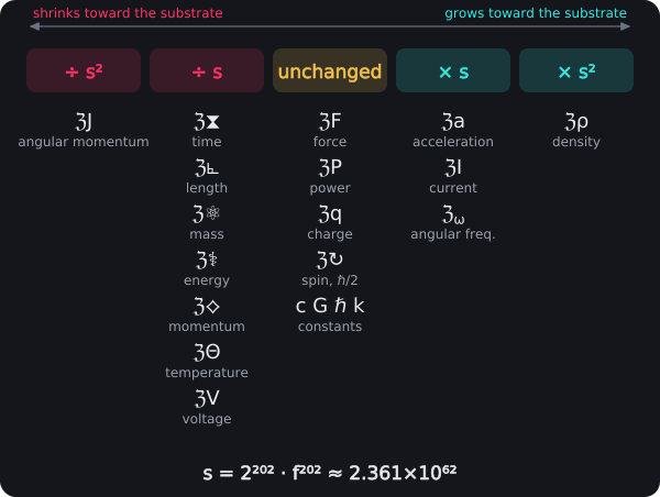
What the Zinf Reduction Scales. Each Zinf unit is its Planck value times a power of s = 2²⁰² · f²⁰². Time, length, mass and energy shrink by s; force, power, charge, spin and the constants stay the same; acceleration and current grow by s, density by s².
This pattern is required by dimensional integrity—not arbitrary but emerging necessarily from holding our constants fixed while rescaling base units. The pattern shows which quantities the reduction leaves unchanged and which it scales; between universes, all of them are set by each universe's level and its parent black hole's singularity.
Z.9 Why Convention C Preserves Physical Law
Applying uniform 1/s scaling to all quantities would break fundamental identities:
- acceleration = length / time² would fail
- power = energy / time would fail
- P = V × I would fail
Convention C (our constants held fixed, base units scaled) preserves every identity and maintains the physical meaning of c, G, ℏ, k_B through the reduction: a retiming and rescaling of clock and ruler from our layer to the Zinf.
Within a universe the constants do not change, and the reduction changes only our measurement scale. Between universes, every Planck value changes with the universe's level and its parent black hole's singularity; ℨ, the reduction of all of them, is the common measure.
Z.10 The Substrate's Extreme Properties and MVU Context
The ℨinf substrate exhibits extreme physical properties emerging naturally from dimensional consistency:
Extraordinarily fast:
- ℨ⧗ ≈ 2.28×10⁻¹⁰⁶ s (about 2 × 10⁶² times faster than Planck time)
- This is the MVU tile τ★ divided by the binary dilation 2^202 and the heritage f^202
Incredibly dense:
- ℨρ ≈ 2.87×10²²¹ kg/m³ (5.6 × 10¹²⁴ times denser than Planck density)
Massively accelerating:
- ℨa ≈ 1.31×10¹¹⁴ m/s² (about 2 × 10⁶² times Planck acceleration)
Enormous current:
- ℨI ≈ 8.21×10⁸⁷ A (about 2 × 10⁶² times Planck current)
Yet unchanged by the reduction:
- Same force: ℨF = F_p ≈ 1.21×10⁴⁴ N
- Same power: ℨP = P_p ≈ 3.63×10⁵² W
- Same charge: ℨq = q_p ≈ 1.88×10⁻¹⁸ C
The MVU-to-Substrate relationship:
- MVU tile (τ★, R★) set by continuum physics bounds ≈ O(1) relative to Planck
- The depth L = 202, read off the universe by the Rupture Rule, amplifies this into the vast substrate hierarchy
- Substrate quantum = MVU tile / (2^L · f^L) ≈ MVU / (2 × 10⁶²)
This combination reveals the substrate as a realm of maximal information density operating at incomprehensible speeds, yet constrained by our constants, held fixed through the reduction. The substrate is not merely "smaller than Planck"—it is the fundamental computational layer where the MVU constraints are satisfied at the deepest recursive level, from which observable reality emerges through 202 levels of binary dilation.
Cross-References:
- Part D: Non-circular derivation of L = 202 from the Rupture Rule, with the tile from MVU constraints
- Part R: UniSpheral growth law, structural capacity scaling, temporal dilation framework
- Z.0: MVU foundation and substrate quantum emergence
- Z.1: Universal scaling principle: the Zinf reduction convention
- Z.2-Z.6: Individual ℨinf units across all physical dimensions
- Z.7: Consistency validation demonstrating dimensional integrity
- Z.8: Interpretation of reduction-invariant versus scaled quantities
References:
Bekenstein, J. D. (1981). Universal upper bound on the entropy-to-energy ratio for bounded systems. Physical Review D, 23(2), 287–298.
Margolus, N., & Levitin, L. B. (1998). The maximum speed of dynamical evolution. Physica D, 120(1–2), 188–195.
Planck, M. (1899). Über irreversible Strahlungsvorgänge. Sitzungsberichte der Königlich Preußischen Akademie der Wissenschaften zu Berlin, 5, 440–480.
Stoney, G. J. (1881). On the physical units of nature. Philosophical Magazine, 11, 381–390.
Wheeler, J. A. (1989). Information, physics, quantum: The search for links. In W. H. Zurek (Ed.), Complexity, entropy, and the physics of information (pp. 3–28). Addison-Wesley.
Z.11 Angular ℨinf Units
Every unit so far has been a scalar or a rate. Spin is neither: it is the one quantity the substrate carries with a direction, and the one the Genesis Prime Pulse inherits rather than generates. It is also the reason Action (𝔸) must be a base dimension rather than a composite of 𝕄, 𝕃 and 𝕋.
ℨinf Spin G
ℨ↻ = ℏ/2 ≈ 5.273×10⁻³⁵ [𝕄·𝕃²·𝕋⁻¹]
Dimensional analysis:
Where (from the book): 2 [∅], ℏ [𝕄·𝕃²·𝕋⁻¹]
[𝕄·𝕃²·𝕋⁻¹]
[𝕄·𝕃²·𝕋⁻¹] ÷ [∅] ≈ [∅] × [∅] = [𝕄·𝕃²·𝕋⁻¹] ≈ [∅] × [∅] = [𝕄·𝕃²·𝕋⁻¹] ≈ [∅]
[𝕄·𝕃²·𝕋⁻¹] = [𝕄·𝕃²·𝕋⁻¹] ≈ [∅] ✓ Valid PulseCore Verified ✓
Spin is unchanged by the reduction, because Action is primitive
Where:
- ℨ↻ [𝕄·𝕃²·𝕋⁻¹] — ℨinf spin quantum; the dimensions of Quantum of Action
- ℏ [𝕄·𝕃²·𝕋⁻¹] — reduced Planck constant, the quantum of action (held at our value under Convention C)
- 2 [∅] — binary half-step, the same 2 that gives ①⥂⧖⌂ = ①⥂⧗⌂/2
Derivation: Spin is quantized in half-integer multiples of the quantum of action. With ℏ held at our value through the reduction and the half-step dimensionless:
ℨ↻ = ℏ/2, unchanged by the reduction
➢ Reduction-invariant result: Spin does not scale with the reduction. It carries the dimensions of action because it is a quantum of action — and action in BPT is a base dimension, not the composite 𝕄·𝕃²·𝕋⁻¹ of conventional physics. That is precisely why spin can stay fixed while mass, length and time all dilate by s: a primitive dimension inherits no scaling from the quantities it is not built from. Where charge is invariant and scalar, spin is invariant and oriented.
ℨinf Mechanical Angular Momentum G
ℨJ = ℏ / s² ≈ 1.892×10⁻¹⁵⁹ [𝕄·𝕃²·𝕋⁻¹]
Dimensional analysis:
Where (from the book): ℏ [𝕄·𝕃²·𝕋⁻¹], s [∅]
[𝕄·𝕃²·𝕋⁻¹]
[𝕄·𝕃²·𝕋⁻¹] ÷ [∅] ≈ [∅] × [∅] = [𝕄·𝕃²·𝕋⁻¹] ≈ [∅] × [∅] = [𝕄·𝕃²·𝕋⁻¹] ≈ [∅]
[𝕄·𝕃²·𝕋⁻¹] = [𝕄·𝕃²·𝕋⁻¹] ≈ [∅] ✓ Valid PulseCore Verified ✓
Mechanical rotation falls by s² at substrate
Where:
- ℨJ [𝕄·𝕃²·𝕋⁻¹] — angular momentum available to one substrate pulse, built from the physical dimensions alone
- ℏ [𝕄·𝕃²·𝕋⁻¹] — quantum of action
- s [∅] — universal scaling factor (2^202 × f^202)
Derivation:
ℨJ = ℨ⚛ × ℨ⦜² / ℨ⧗
= (m_p/s) × (ℓ_p/s)² / (t_p/s)
= (m_p·ℓ_p²/t_p) / s²
= ℏ / s²
Consistency check: ℨρ × ℨJ = (ρ_p × s²) × (ℏ / s²) = ρ_p·ℏ ✓ — the two scalings are reciprocal
➢ This is a different quantity from ℨ↻, not a contradiction with it. Built from 𝕄, 𝕃 and 𝕋 alone, it inherits their dilation and falls by s². Where density gains the factor s², mechanical rotation loses it: the substrate is maximally dense and minimally rotational, and the product of the two is unchanged by the reduction.
Spin Is Not a Property of One Pulse G
ℨ↻ = ℨJ × (s²/2)
Dimensional analysis:
[𝕄·𝕃²·𝕋⁻¹]
[𝕄·𝕃²·𝕋⁻¹] × ([∅] ÷ [∅]) = [𝕄·𝕃²·𝕋⁻¹] × [∅] = [𝕄·𝕃²·𝕋⁻¹]
[𝕄·𝕃²·𝕋⁻¹] = [𝕄·𝕃²·𝕋⁻¹] ✓ Valid PulseCore Verified ✓
Spin is mechanical rotation carrying Complete Computational Action
Where:
- ℨ↻ [𝕄·𝕃²·𝕋⁻¹] — the spin quantum, ℏ/2
- ℨJ [𝕄·𝕃²·𝕋⁻¹] — mechanical angular momentum of one pulse, ℏ/s²
- s²/2 [ℨ·ↁ·𝔸] — Complete Computational Action; magnitude s²/2 ≈ 2.787×10¹²⁴ coherent substrate operations per spin quantum
Derivation:
ℨ↻ / ℨJ = (ℏ/2) / (ℏ/s²) = s²/2 ≈ 2.787×10¹²⁴
Equivalence check: [ℨ·ↁ·𝔸] ⇔ [∅] = [ℨ·ↁ·𝔸] ✓ — under the equivalence rule (combine unique dimensions), pairing a dimension with the dimensionless yields no reduction — the residue stands.
The residue is not dimensionless. [ℨ·ↁ·𝔸] is a named composite of the BPT basis — Complete Computational Action — so the factor separating spin from mechanical rotation is not a bare count but a computational act: substrate, data operation and action together. Its magnitude is s²/2; its dimension is the work of computing.
➢ A single pulse cannot carry spin-½; it is s²/2 times too small. Spin is therefore not intrinsic to a pulse but a collective property of a whole recursive structure — which is why it is quantized at all, since the substrate cannot deliver a fraction of s²/2 coordinated pulses. Action is the cost of an operation, so 𝔸 never appears without ↁ: there is no price without a transaction. Charge attaches to a pulse. Spin attaches to a spiral.
Substrate Angular Frequency Ceiling
ℨ_ω = 1 / ℨ⧗ ≈ 4.379×10¹⁰⁵ s⁻¹
Dimensional analysis:
[ℨ]
[∅] ÷ [𝕋] = [𝕋⁻¹]
[ℨ] = [𝕋⁻¹] ✓ Valid PulseCore Verified ✓
The fastest rotation the substrate can represent
Where:
- ℨ_ω [𝕋⁻¹] — substrate angular frequency; one full phase advance per substrate tick
- ℨ⧗ [𝕋] — substrate temporal quantum, ①⥂⧗⌂/s ≈ 2.283×10⁻¹⁰⁶ s (Z.1)
- ⯴ [𝕋⁻¹] — Local Harmonic Amplifier, defined in the section that follows
Consistency check: ⯴ × ℨ⧗ = 1, therefore ⯴ = 1/ℨ⧗ = ℨ_ω ✓ — the amplifier and the angular ceiling are the same constant
➢ Spin needs a rate as well as a magnitude, and the substrate supplies a hard ceiling: nothing can turn faster than one phase step per ℨ⧗. That ceiling is numerically identical to the Local Harmonic Amplifier ⯴ introduced in the next section — the same constant read two ways. As a clock rate it normalizes substrate time to unity; as an angular frequency it bounds every rotation in the hierarchy. Spin is quantized in magnitude by s²/2 and bounded in rate by ℨ_ω.
Local Harmonic Amplifier - Computational Normalization Constant
Variable Definition
Symbol: ⯴
Name: Local Harmonic Amplifier
Long Form: local_harmonic_amplifier
Quality: Computational normalization constant
Dimensions: [𝕋⁻¹]
Value: 4.379×10¹⁰⁵ s⁻¹
Physical Significance
The Local Harmonic Amplifier represents the fundamental frequency scale required to normalize substrate temporal quanta to unity at our observational level (Level 202). It bridges the computational substrate operating at ℨ⧗ ≈ 2.283×10⁻¹⁰⁶ seconds with practical calculations requiring normalized unity reference frames.
Harmonic Zinf Normalization Relationship G
⯴ × ℨ⧗ = ⚚ℨ = 1
Dimensional analysis:
[𝕋⁻¹] × [𝕋] = [∅]
[ℨ]
[∅]
[∅] = [ℨ] = [∅] ✓ Valid PulseCore Verified ✓
Substrate temporal quantum normalized to unity for Level 202 calculations
Where:
- ⯴ [𝕋⁻¹] — Local Harmonic Amplifier; normalization frequency for substrate temporal quantum
- ℨ⧗ [𝕋] — Zinf temporal quantum; fundamental substrate full-pulse duration ≈ 2.283×10⁻¹⁰⁶ s
- ⚚ℨ [∅] — Harmonic Zinf; normalized dimensionless temporal reference equal to unity
- 1 [∅] — unity normalization target; computational reference frame at observational level
➢ The Local Harmonic Amplifier enables computational normalization by establishing the precise frequency scaling that transforms substrate temporal quanta into a unity reference frame at Level 202, facilitating practical calculations across the 62-order-of-magnitude gap between Planck-scale observations and substrate computational architecture.
Non-Circular Derivation
The amplifier emerges directly from the substrate temporal quantum derived in Part D, with L from the Rupture Rule and no arbitrary normalization choices.
Computational Chain
Base relationship:
ℨ⧗ = ①⥂⧗⌂ / (2^L · f^L), with L = 202
Substituting values:
ℨ⧗ = 5.39124760×10⁻⁴⁴ s / (2²⁰² · f²⁰²) ≈ 2.283×10⁻¹⁰⁶ s
Local Harmonic Amplifier:
⯴ = 1 / ℨ⧗ = (2²⁰² · f²⁰²) / 5.39124760×10⁻⁴⁴ s ≈ 4.379×10¹⁰⁵ s⁻¹
Normalization:
⯴ × ℨ⧗ = 1 (exact)
Step 1: Substrate Temporal Quantum from MVU Convergence
From Part D (Minimum Viable Universe derivation):
- τ★ = t_p · √(π/(χ★ ln2)) (MVU tile from constraint convergence)
- L = 202 (from the Rupture Rule, L = log₂(t↯ / ①⥂⧗⌂))
- ℨ⧗ = ①⥂⧗⌂ / (2^L · f^L) = s▱ · τ★ / (2^L · f^L) (substrate quantum)
Numerical evaluation:
ℨ⧗ = 5.391×10⁻⁴⁴ s / (2²⁰² · f²⁰²)
ℨ⧗ ≈ 2.283×10⁻¹⁰⁶ seconds
This value is derived from first-principles physics (Bekenstein bound, Margolus-Levitin theorem, causality, Schwarzschild threshold) combined with the depth L from the Rupture Rule - the universe's age at rupture counted in its own Planck pulses.
Step 2: Amplifier as Normalization Frequency
To enable computational operations at Level 202 using normalized unity references, define:
⯴ = 1 / ℨ⧗ = ℨ∞
Dimensional analysis:
[𝕋⁻¹]
[∅] ÷ [𝕋] = [𝕋⁻¹]
[ℨ⁻¹]
[𝕋⁻¹] = [𝕋⁻¹] = [ℨ⁻¹] ✓ Valid PulseCore Verified ✓
Amplifier equals Zinfinity frequency
Where:
- ⯴ [𝕋⁻¹] — Local Harmonic Amplifier
- ℨ⧗ [𝕋] — substrate temporal quantum
- ℨ∞ [ℨ⁻¹] — Zinfinity frequency from Part Z
Numerical evaluation:
⯴ = 1 / (2.283×10⁻¹⁰⁶ s)
⯴ ≈ 4.379×10¹⁰⁵ s⁻¹
Critical insight: The Local Harmonic Amplifier is not an independent constant but the direct reciprocal of the substrate temporal quantum. It represents the fundamental oscillation frequency at Level 0 - the rate at which substrate pulses complete full binary cycles (0→1→0).
Step 3: Relationship to Universal Scaling Factor
The amplifier connects to the universal scaling factor s = 2^202 · f^202 through:
⯴ = (2^L · f^L) / ①⥂⧗⌂
Dimensional analysis:
Where (from the book): L [∅], 2^L [∅]
[𝕋⁻¹]
([∅] × [∅]^([∅])) ÷ [𝕋] = ([∅] × [∅]) ÷ [𝕋] = [∅] ÷ [𝕋] = [𝕋⁻¹]
[𝕋⁻¹] = [𝕋⁻¹] ✓ Valid PulseCore Verified ✓
Amplifier from binary dilation and Planck time
Where:
- ⯴ [𝕋⁻¹] — Local Harmonic Amplifier
- L [∅] — dilation depth; L = 202
- 2^L · f^L [∅] — universal scaling factor; s = 2²⁰² · f²⁰²
- ①⥂⧗⌂ [𝕋] — Local Pulse Tempo (Planck time) at Level 202
Derivation:
⯴ = 1 / ℨ⧗
= 1 / (①⥂⧗⌂ / (2^L · f^L))
= (2^L · f^L) / ①⥂⧗⌂
= (2²⁰² · f²⁰²) / (5.391×10⁻⁴⁴ s)
≈ 4.379×10¹⁰⁵ s⁻¹
➢ This demonstrates that the Local Harmonic Amplifier emerges naturally from the binary dilation structure, representing how many substrate cycles occur per Planck time unit at our observational level.
Computational Implementation
Precision Considerations
When implementing BPT calculations spanning 106 orders of magnitude (from ℨ to one second), the normalized reference frame eliminates numerical instabilities:
Standard approach (problematic):
Calculate with ℨ⧗ ≈ 1×10⁻¹⁰⁶ s
Requires extended precision arithmetic
Accumulated floating-point errors across deep recursion
Normalized approach (stable):
Set ⚚ℨ = ⯴ × ℨ⧗ = 1 (dimensionless unity)
All substrate calculations in normalized units
Convert to SI only for final observables
Harmonic Normalization Identity G
⚚ℨ = ⯴ × ℨ⧗ ≡ 1
Dimensional analysis:
[ℨ]
[𝕋⁻¹] × [𝕋] ≡ [∅] = [∅] ≡ [∅]
[ℨ] = [∅] ≡ [∅] ✓ Valid PulseCore Verified ✓
Normalized substrate temporal reference for Level 202
Where:
- ⚚ℨ [∅] — Harmonic Zinf; normalized dimensionless temporal quantum
- ⯴ [𝕋⁻¹] — Local Harmonic Amplifier (4.379×10¹⁰⁵ s⁻¹)
- ℨ⧗ [𝕋] — substrate temporal quantum (2.283×10⁻¹⁰⁶ s)
- ≡ 1 [∅] — identity normalization; computational unity reference
➢ The Harmonic Zinf ⚚ℨ = 1 establishes a normalized computational reference frame where substrate temporal operations equal unity, enabling stable numerical calculations across the recursive hierarchy while maintaining exact dimensional consistency with physical substrate quantum ℨ⧗ when converted back to SI units.
Physical Interpretation
The Local Harmonic Amplifier is not an arbitrary normalization choice but represents fundamental computational architecture:
As substrate frequency:
- ⯴ = ℨ∞ ≈ 4.38×10¹⁰⁵ cycles per second
- The rate at which Level 0 completes full binary cycles (0→1→0)
- Operating frequency of the primordial computational engine
As normalization constant:
- Bridges about 62 orders of magnitude between substrate and Planck observation
- Enables practical calculations at Level 202
- Maintains dimensional consistency across recursive hierarchy
As universal clock rate:
- Every physical process at every layer reduces to substrate cycles
- Observable phenomena = integer multiples of ℨ⧗
- The amplifier converts these back to normalized unity reference
Relationship to Other BPT Constants
Connection to Universal Scaling Factor:
⯴ = s / ①⥂⧗⌂
where s = 2²⁰² · f²⁰² (L = 202 from the Rupture Rule)
Connection to Harmonic Number:
⯴ / ⚚⌂ = 1 / ①⥂⧗⌂
where ⚚⌂ = s (ℨ∞ / s ≈ 1.855 × 10⁴³ s⁻¹, the Planck frequency)
Connection to Planck Frequency:
⯴ = ν_p × 2^L × f^L
where ν_p = 1/①⥂⧗⌂ ≈ 1.855 × 10⁴³ s⁻¹ (the Planck frequency, one full Tempo)
All relationships follow directly from the non-circular MVU derivation - the amplifier contains no free parameters.
Why This Matters
The Local Harmonic Amplifier addresses a fundamental computational challenge: how to perform calculations at substrate scale using finite-precision arithmetic. By establishing ⚚ℨ = 1 as the normalized reference, all BPT computations become:
- Numerically stable - no extreme exponents in intermediate steps
- Dimensionally consistent - converts cleanly to SI when needed
- Physically meaningful - represents actual substrate oscillation frequency
This is not "inventing a constant to fit data" but recognizing that substrate frequency and normalization factor are the same physical quantity viewed from different computational perspectives.
Cross-References:
- Part D: Non-circular derivation of ℨ⧗ from MVU constraints
- Part Z: Complete ℨinf unit system with ℨ∞ = 1/ℨ⧗
- Z.2: Substrate temporal quantum ℨ⧗ ≈ 2.283×10⁻¹⁰⁶ s
- Z.4: Power and force unchanged by the reduction
Computational Note: While ⚚ℨ = 1 is mathematically exact by definition, practical implementations should verify:
|⯴ × ℨ⧗ - 1| < machine_epsilon
to ensure numerical precision across deep recursive calculations.
The Harmonic Amplifier - Universal Normalization Across Dimensions
Core Concept: Computational Normalization
The Harmonic Amplifier is a fundamental computational tool in Binary Pulse Theory that enables normalized calculations across the vast hierarchy separating substrate (Level 0) from observation (Level 202). When working with substrate units that are ~2 × 10⁶² times smaller than Planck scale, direct numerical computation becomes unstable due to extreme exponents. The Harmonic Amplifier solves this by establishing normalized unity references for each physical dimension.
The central principle: For any physical quantity Q, define its Harmonic Amplifier as:
Universal Harmonic Amplifier Definition G
⯴_Q ≡ 1 / Q▱
Normalization constant for physical dimension Q (always the reciprocal of the substrate value)
In terms of Planck-layer quantities Q_p and the binary factor s = 2^L · f^L:
- If Q scales down: Q▱ = Q_p / s ⇒ ⯴_Q = s / Q_p
- If Q is invariant: Q▱ = Q_p ⇒ ⯴_Q = 1 / Q_p
- If Q scales up by s: Q▱ = Q_p · s ⇒ ⯴_Q = 1 / (s · Q_p)
- If Q scales up by s²: Q▱ = Q_p · s² ⇒ ⯴_Q = 1 / (s² · Q_p)
Normalization identity (all cases):
⯴_Q × Q▱ = 1
➢ The Harmonic Amplifier establishes a universal methodology for normalizing any physical quantity to computational unity, enabling stable numerical operations across the 62 orders of magnitude between substrate and Planck scale while maintaining exact dimensional consistency when converting back to SI units.
Why Multiple Amplifiers Are Needed
Different physical dimensions scale differently through the recursive hierarchy (Part Z). With our constants (c, G, ℏ, k_B) held fixed through the reduction, base units scale according to their dimensional structure:
Scaling Categories:
- Down by 1/s: Time, length, mass, energy, temperature, voltage
- Unchanged: Force, power, charge, our constants
- Up by s: Acceleration, current
- Up by s²: Density
Each scaling category requires its own amplifier to achieve proper normalization. However, spacetime (time + length) forms the fundamental pair - all other amplifiers derive from these two through dimensional relationships.
The Two Fundamental Amplifiers
Temporal Harmonic Amplifier G
⯴_t = (2^L · f^L) / ①⥂⧗⌂ = ℨ∞
Dimensional analysis:
Where (from the book): L [∅], 2^L [∅]
[𝕋⁻¹]
([∅] × [∅]^([∅])) ÷ [𝕋] = ([∅] × [∅]) ÷ [𝕋] = [∅] ÷ [𝕋] = [𝕋⁻¹]
[ℨ⁻¹]
[𝕋⁻¹] = [𝕋⁻¹] = [ℨ⁻¹] ✓ Valid PulseCore Verified ✓
Fundamental oscillation frequency at substrate Level 0
Where:
- ⯴_t [𝕋⁻¹] — Temporal Harmonic Amplifier; normalization frequency for time
- ①⥂⧗⌂ [𝕋] — Local Pulse Tempo (Planck time) at Level 202 (5.391×10⁻⁴⁴ s)
- ℨ∞ [ℨ⁻¹] — Zinfinity frequency from Part Z
- L [∅] — Dilation depth; L = 202
- 2^L · f^L [∅] — Binary scaling factor; s = 2²⁰² · f²⁰²
Normalization identity:
⯴_t × ℨ⧗ = 1
Numerical value (Level 202):
⯴_t = (2²⁰² · f²⁰²) / (5.391×10⁻⁴⁴ s) ≈ 4.379×10¹⁰⁵ s⁻¹
Physical meaning: ⯴_t represents the substrate oscillation frequency - the rate at which Level 0 completes full binary cycles (0→1→0). Every physical process at every layer ultimately reduces to integer multiples of this fundamental computational clock rate.
➢ The Temporal Harmonic Amplifier is identical to the Zinfinity frequency ℨ∞ derived in Part Z, demonstrating that "amplifier" and "substrate frequency" are the same physical quantity viewed from different computational perspectives - one emphasizes normalization utility, the other emphasizes oscillation physics.
Spatial Harmonic Amplifier G
⯴_s = (2^L · f^L) / l_p
Dimensional analysis:
Where (from the book): L [∅], 2^L [∅]
[𝕃⁻¹]
([∅] × [∅]^([∅])) ÷ [𝕃] = ([∅] × [∅]) ÷ [𝕃] = [∅] ÷ [𝕃] = [𝕃⁻¹]
[𝕃⁻¹] = [𝕃⁻¹] ✓ Valid PulseCore Verified ✓
Fundamental wavenumber at substrate Level 0
Where:
- ⯴_s [𝕃⁻¹] — Spatial Harmonic Amplifier; normalization wavenumber for length
- l_p [𝕃] — Planck length at Level 202 (1.616×10⁻³⁵ m)
- L [∅] — Dilation depth; L = 202
- 2^L · f^L [∅] — Binary scaling factor; s = 2²⁰² · f²⁰²
Normalization identity:
⯴_s × ℨ⦜ = 1
Numerical value (Level 202):
⯴_s = (2²⁰² · f²⁰²) / (1.616×10⁻³⁵ m) ≈ 1.461×10⁹⁷ m⁻¹
Physical meaning: ⯴_s represents the substrate wavenumber - how many spatial pixels fit into one unit of Planck length. This is the fundamental "grid resolution" of spacetime at Level 0.
➢ The Spatial Harmonic Amplifier establishes the fundamental spatial frequency of the computational substrate, representing the pixel density of reality at the deepest recursive level where spacetime tessellation occurs through binary subdivision.
Coupling Between Temporal and Spatial Amplifiers
In our universe (Level 202), where Diameter = 𝒞→ × Rhythm and the reduction to Zinf units holds c at our value (Convention C from Part Z), the two fundamental amplifiers are coupled:
Light Speed Coupling G
⯴_t = 𝒞→ × ⯴_s
Dimensional analysis:
[𝕋⁻¹]
[𝕃·𝕋⁻¹] × [𝕃⁻¹] = [𝕋⁻¹]
[𝕋⁻¹] = [𝕋⁻¹] ✓ Valid PulseCore Verified ✓
Relativistic coupling of temporal and spatial amplifiers
Where:
- ⯴_t [𝕋⁻¹] — Temporal Harmonic Amplifier
- ⯴_s [𝕃⁻¹] — Spatial Harmonic Amplifier
- 𝒞→ [𝕃·𝕋⁻¹] — Speed of light; our value, fixed within our universe (2.998×10⁸ m/s)
Derivation:
⯴_t / ⯴_s = ((2^L · f^L) / t_p) / ((2^L · f^L) / l_p)
= l_p / t_p
= c (by definition of Planck length)
Therefore: ⯴_t = 𝒞→ × ⯴_s
Verification (Level 202):
𝒞→ × ⯴_s = (2.998×10⁸ m/s) × (1.461×10⁹⁷ m⁻¹) ≈ 4.38×10¹⁰⁵ s⁻¹ ≈ ⯴_t ✓
➢ Within any universe, where 𝒞→ is fixed, the temporal and spatial amplifiers maintain a fixed ratio equal to that universe's 𝒞→, ensuring relativistic consistency where ℨ⧗ and ℨ⦜ scale together through identical binary dilation, preserving the spacetime metric through the reduction.
Critical insight: This coupling is not accidental - it follows from Diameter = 𝒞→ × Rhythm and Convention C (our constants held fixed through the reduction). The two amplifiers are not independent but linked by the same 𝒞→ that governs electromagnetic propagation, demonstrating deep unity between computational normalization and physical law.
Derived Amplifiers for Other Dimensions
Once temporal and spatial amplifiers are established, amplifiers for other physical quantities follow from dimensional relationships:
Mass Amplifier G
⯴_m = (2^L · f^L) / m_p
Dimensional analysis:
Where (from the book): ⯴_m [𝕄⁻¹]
[𝕄⁻¹]
([∅]^([∅]) × [∅]^([∅])) ÷ [𝕄] = ([∅] × [∅]^([∅])) ÷ [𝕄] = ([∅] × [∅]) ÷ [𝕄] = [∅] ÷ [𝕄] = [𝕄⁻¹]
[𝕄⁻¹] = [𝕄⁻¹] ✓ Valid PulseCore Verified ✓
Mass normalization for substrate quantum
Where:
- ⯴_m [𝕄⁻¹] — Mass Harmonic Amplifier
- m_p [𝕄] — Planck mass (2.176×10⁻⁸ kg)
Normalization: ⯴_m × ℨ⚛ = 1
Energy Amplifier G
⯴_E = (2^L · f^L) / E_p
Dimensional analysis:
Where (from the book): ⯴_E [𝕄⁻¹·𝕃⁻²·𝕋²]
[𝕄⁻¹·𝕃⁻²·𝕋²]
([∅]^([∅]) × [∅]^([∅])) ÷ [𝕄·𝕃²·𝕋⁻²] = ([∅] × [∅]^([∅])) ÷ [𝕄·𝕃²·𝕋⁻²] = ([∅] × [∅]) ÷ [𝕄·𝕃²·𝕋⁻²] = [∅] ÷ [𝕄·𝕃²·𝕋⁻²] = [𝕄⁻¹·𝕃⁻²·𝕋²]
[𝕄⁻¹·𝕃⁻²·𝕋²] = [𝕄⁻¹·𝕃⁻²·𝕋²] ✓ Valid PulseCore Verified ✓
Energy normalization for substrate quantum
Where:
- ⯴_E [𝕄⁻¹·𝕃⁻²·𝕋²] — Energy Harmonic Amplifier
- E_p [𝕄·𝕃²·𝕋⁻²] — Planck energy
Normalization: ⯴_E × ℨ⚕ = 1
Relationship: ⯴_E = ⯴_m / 𝒞→² (from E = mc²)
Temperature Amplifier G
⯴_T = (2^L · f^L) / T_p
Dimensional analysis:
Where (from the book): ⯴_T [Θ⁻¹], T_p [Θ]
[Θ⁻¹]
([∅]^([∅]) × [∅]^([∅])) ÷ [Θ] = ([∅] × [∅]^([∅])) ÷ [Θ] = ([∅] × [∅]) ÷ [Θ] = [∅] ÷ [Θ] = [Θ⁻¹]
[Θ⁻¹] = [Θ⁻¹] ✓ Valid PulseCore Verified ✓
Temperature normalization for substrate quantum
Where:
- ⯴_T [Θ⁻¹] — Temperature Harmonic Amplifier
- T_p [Θ] — Planck temperature
Normalization: ⯴_T × ℨΘ = 1
Relationship: ⯴_T = k_B × ⯴_E (from E = k_BT with k_B held at our value)
Note on invariant quantities: Dimensions the reduction does not scale (force, power, charge) have ⯴_Q = 1 / Q_p, since Q▱ = Q_p.
Universal Amplification Methodology Across Harmonic Levels
The amplifier derivation process represents a universal methodology applicable at any harmonic level n, not just our Level 202. Any observer at any layer can define their own normalized reference frame.
General Amplifier at Arbitrary Level G
For an observer at level n with scale factor s_n = 2^n · f^n:
- If Q▱(n) = Q⌾(n) / s_n ⇒ ⯴_Q(n) = s_n / Q⌾(n)
- If Q▱(n) = Q⌾(n) ⇒ ⯴_Q(n) = 1 / Q⌾(n)
- If Q▱(n) = Q⌾(n) · s_n ⇒ ⯴_Q(n) = 1 / (s_n · Q⌾(n))
- If Q▱(n) = Q⌾(n) · s_n² ⇒ ⯴_Q(n) = 1 / (s_n² · Q⌾(n))
Normalization: ⯴_Q(n) × Q▱(n) = 1
Universal properties:
- Binary scaling law: Factor of 2 per level (from Prime Pulse two-phase structure)
- Normalization goal: All observers can achieve Q▱ × ⯴_Q = 1
- Relativistic coupling: within each universe, ⯴_t(n) = 𝒞→(n) × ⯴_s(n), with 𝒞→(n) that universe's own light speed
- Dimensional consistency: Derived amplifiers relate through physical law
➢ The amplification methodology is a meta-constant - a universal procedure that generates level-specific normalization constants while maintaining theoretical unity across all harmonic positions, enabling any observer to bridge their local observables to substrate fundamentals.
Why This Is Not Arbitrary
The Harmonic Amplifier might appear to be "just unit conversion," but it represents fundamental physics:
- It equals substrate frequency: ⯴_t = ℨ∞ (substrate oscillation rate)
- It reflects recursion depth: ⯴ ∝ 2^L (the depth L of the Rupture Rule)
- It enables predictions: Knowing ⯴ lets you calculate substrate properties
- It's measurable: In principle, can be determined from Planck-scale experiments
The amplifier is not tuned to fit data - it emerges directly from:
- MVU constraint convergence (Part D)
- The Rupture Rule (L = 202, the universe's age at rupture in its own Planck pulses)
- Binary dilation architecture (s = 2^202 · f^202, one doubling with heritage per level)
Divergence in Child Universes (Modified Constants)
In child universes spawned from Null Wells, every Planck value, 𝒞→ included, is set by the child's level and its parent black hole's singularity (the spin that sets its heritage f via ⟪C⟫). With these modified constants (Chapter 2), the coupling between temporal and spatial amplifiers can differ:
Modified Constant Universe G
⯴'_t = 𝒞→' × ⯴'_s
Dimensional analysis:
[𝕋⁻¹]
[𝕃·𝕋⁻¹] × [𝕃⁻¹] = [𝕋⁻¹]
[𝕋⁻¹] = [𝕋⁻¹] ✓ Valid PulseCore Verified ✓
Amplifier coupling with density-modified light speed
Where:
- ⯴'_t [𝕋⁻¹] — Temporal amplifier in child universe
- ⯴'_s [𝕃⁻¹] — Spatial amplifier in child universe
- 𝒞→' [𝕃·𝕋⁻¹] — Density-modified light speed (from Chapter 2 scaling functions)
When 𝒞→' ≠ 𝒞→:
- Time and space no longer scale identically
- ⯴'_t / ⯴'_s ≠ 𝒞→ (our universe value)
- Different physics emerges in child universe
Example: If child universe has 𝒞→' = 0.5𝒞→ (slower light):
⯴'_t = 0.5𝒞→ × ⯴'_s
→ Either time dilates faster or space dilates slower
→ Different causal structure than parent universe
➢ Density-modified constants in child universes (from Null Well parameter inheritance) can break the standard temporal-spatial amplifier coupling, producing domains where spacetime geometry differs fundamentally from our Level 202 physics while still operating on the same substrate computational architecture.
This demonstrates that while the amplification methodology is universal (every universe can normalize to unity), the specific amplifier values and their relationships vary based on inherited modified constants, creating the diverse multiverse landscape predicted by BPT's universe classification framework.
Cross-References:
- Part D: Non-circular derivation of L = 202 from the Rupture Rule and ℨ⧗ from MVU constraints
- Part Z: Complete ℨinf unit system showing all dimensional scaling categories
- Chapter 2: Null Well parameter inheritance and density-modified constants
- Z.4: Force and power unchanged by the reduction
- Z.8: Reduction-invariant vs scaled quantity classification
The Universe and The UniSphere: Pulse Rhythm, Data Energy, and Light Speed
The constants of physics are not inexplicable inputs but derived harmonics of the Zinf ℨ seed constant. From the primordial tick ℨ emerges the UniSphereal Pulse Tempo, the first stable binary cycle of the cosmos. Through recursive scaling, this seed extends outward until, at our universe's harmonic level, it produces the temporal and energetic constants we observe in our local universe.
Pulse Rhythm
The Universe and The UniSphere
UniSpheral Pulse Tempo G
☫⥂ = ℨ ≈ 2.283 × 10⁻¹⁰⁶ seconds
The primordial temporal quantum at the UniSphereal level.
Where:
- ☫⥂ [𝕋] – UniSphereal Pulse Tempo; first stable binary cycle duration at primordial level
- ℨ [ℨ] – Zinf Unit seed constant; the Zinf's full cycle (0→1→0), two data rhythms ↁℨ⧖
- 2.283 × 10⁻¹⁰⁶ [𝕋] – approximate numerical value in seconds
➢ The primordial temporal quantum at the UniSphereal level, representing the first stable binary cycle that emerged from the original void and serves as the root frequency from which all subsequent temporal harmonics derive.
Local Universe Pulse Tempo G
⥂⌂ ≈ ☫⥂ × 2²⁰² × f²⁰² ≈ 5.39 × 10⁻⁴⁴ seconds
Where:
- ⥂⌂ [𝕋] – Local Pulse Tempo; temporal quantum at our universe level 202
- ☫⥂ [𝕋] – UniSphereal Pulse Tempo; primordial binary cycle duration
- 2²⁰² [∅] – harmonic scaling factor; exponential amplification across 202 levels
- f²⁰² [∅] – null-well heritage across 202 levels; f ≈ 1.018, f²⁰² ≈ 36.73
- 5.39 × 10⁻⁴⁴ [𝕋] – approximate numerical value in seconds (Planck time)
➢ The fundamental temporal constants emerge through harmonic scaling from the primordial UniSphereal level to our local universe at level 202, revealing the computational hierarchy underlying observed Planck time.
The Speed of Light
The Universe and The UniSphere
UniSpheral Speed of Light G
𝒞→☫ = 2☫⊕ / ☫⥂
Where:
- 𝒞→☫ [𝕃·𝕋⁻¹] – UniSphereal speed of light; fundamental velocity limit at primordial computational level
- ☫⊕ [𝕃] – UniSphereal Pulse Diameter; fundamental spatial quantum at primordial level
- ☫⥂ [𝕋] – UniSphereal Pulse Tempo; complete binary cycle duration (= ℨ)
- 2 [∅] – binary cycle multiplier; accounts for full oscillation distance
Dimensional analysis:
Where (from the book): 2 [∅]
[𝕃·𝕋⁻¹]
[∅] × [𝕃] ÷ [𝕋] = [𝕃] ÷ [𝕋] = [𝕃·𝕋⁻¹]
[𝕃·𝕋⁻¹] = [𝕃·𝕋⁻¹] ✓ Valid PulseCore Verified ✓
➢ The primordial speed of light at the UniSphereal level, establishing the fundamental velocity limit that governs information propagation at the root computational layer. In the Zinf unit system ☫⊕ = 𝒞→ · ℨ/2, so 𝒞→☫ equals 𝒞→: at the root, data and light move together. Data keeps that clock, one step every Zinf Rhythm ↁℨ⧖ in every universe, with no interference, so at level L its speed is the local Diameter per Zinf Rhythm, vↁ = 𝒞→ · (2f)^L, about 2.36 × 10⁶² 𝒞→ ≈ 7.08 × 10⁷⁰ m/s in ours; light and everything physical stay capped at 𝒞→.
Local Universe Speed of Light G
𝒞→⌂ = 2⊕⌂ / ①⥂⧗⌂ = 2⊕(202) / (2²⁰² × f²⁰² × ℨ)
Where:
- 𝒞→⌂ [𝕃·𝕋⁻¹] – Local speed of light; velocity limit in our observed universe
- ⊕⌂ [𝕃] – Local Pulse Diameter; spatial quantum at our harmonic level
- ⥂⌂ [𝕋] – Local Pulse Tempo; complete binary cycle at our universe level
- ⊕(202) [𝕃] – Pulse Diameter at our harmonic level
- 2²⁰² [∅] – harmonic scaling factor; binary amplification across 202 levels
- ℨ [ℨ] – Zinf Unit; fundamental temporal atom and scaling foundation
- 2 [∅] – binary cycle multiplier; accounts for full oscillation distance
Dimensional analysis:
Where (from the book): 2 [∅], 𝒞→⌂ [𝕃·𝕋⁻¹], ⊕⌂ [𝕃], ⊕(202) [𝕃], 2²⁰² [∅], ℨ [𝕋]
[𝕃·𝕋⁻¹]
[∅] × [𝕃] ÷ [𝕋] = [𝕃] ÷ [𝕋] = [𝕃·𝕋⁻¹]
[∅] × [𝕃] ÷ ([∅] × [𝕋]) = [𝕃] ÷ ([∅] × [𝕋]) = [𝕃] ÷ [𝕋] = [𝕃·𝕋⁻¹]
[𝕃·𝕋⁻¹] = [𝕃·𝕋⁻¹] = [𝕃·𝕋⁻¹] ✓ Valid PulseCore Verified ✓
➢ The speed of light emerges as a derived constant from the fundamental relationship between local Pulse Diameter and harmonically scaled temporal quantum, revealing that 𝒞→ is not arbitrary but determined by our position at our harmonic level and by our parent black hole's singularity, which together set every Planck value of a universe. Within our universe 𝒞→ is fixed.
Zinf Scaling Zinf Scaled Data-Physical Conversion
The transformation from single-transition Data to complete-cycle Physical occurs through systematic substrate operations:
Zinf Scaled Data-Physical Conversion Mechanism
⩈(ℨ): ↁ(⧖) ⧉ ↁ̄(⧖) → ⚛(①⥂)
Dimensional analysis:
Where (from the book): Γ(ℨ) [∅], ↁ(⧖) [1ᵇ], ↁ̄(⧖) [1ᵇ], ⚛(⥂) [∅]
[∅]([ℨ]) : [1ᵇ] ⧉ [1ᵇ] → [ℨ·ↁ·𝔸·𝕄·𝕃]([ℨ]) = [∅] : [1ᵇ] ⧉ [1ᵇ] → [ℨ·ↁ·𝔸·𝕄·𝕃]([ℨ]) = [∅] : [1ᵇ] ⧉ [1ᵇ] → [ℨ·ↁ·𝔸·𝕄·𝕃] ✓ Valid PulseCore Verified ✓
Process by which Data fundamentals combine into Physical manifestations
Where:
- Γ(ℨ) [∅] – Zinf-scaled conversion coupling function
- ↁ(⧖) [1ᵇ] – Data fundamental from first transition at Time Crystal scale
- ↁ̄(⧖) [1ᵇ] – Data fundamental from return transition at Time Crystal scale
- ⧉ [∅] – Data combination operator (computational fusion)
- ⚛(⥂) [∅] – Physical fundamental manifested at Pulse Rate scale
- → – Conversion process operator
➢ The conversion mechanism demonstrates how two Data fundamentals (representing forward and return transitions) combine through computational fusion to manifest as single Physical fundamentals operating at twice the temporal scale. This process preserves all computational information while adding dimensional properties through cyclical completion.
1.6 Testable Predictions
- Temporal Quantization at ℨ Scale: High-precision atomic clocks should reveal synchronization limits at ℨ ≈ 2.283 × 10⁻¹⁰⁶ seconds, detectable through quantum tunneling rate analysis and coherent control experiments.
- Harmonic Scaling in Physical Constants: Fundamental constants should exhibit relationships following ①⥂⧖(n) = ℨ × 2ⁿ × fⁿ / 2, verifiable through precision measurements of Planck units and dimensionless constants.
- Cosmological ℨ Signatures: Cosmic microwave background should show anisotropies at ℨ scales with periodicity matching harmonic progression 2ⁿ × fⁿ × ℨ, detectable through ultra-high precision CMB analysis.
- Information Processing Limits: Quantum computers should encounter fundamental limits at 1 bit per Zinf Rhythm ↁℨ⧖ (2 bits per ℨ) processing rate, testable through quantum algorithm optimization and computational complexity analysis.
These discoveries validate the computational foundation of reality and enable technologies operating at cosmic frame rates, potentially including temporal manipulation devices and information-based energy generation systems.