Chapter 3 · Section 1
From Binary Transition to Physical Energy — The UniSpheral Data Spectrum
What if energy isn't fundamental but emerges from computational processes? The Base Calculation proposes that binary state transitions generate measurable physical energy through mathematically defined mechanisms, offering a computational foundation for energy generation processes (Bennett, 1973; Fredkin, 2003). This reframes long-held physics assumptions about the nature of energy itself.
Data in the UniSphere
In the UniSphere, data is not symbolic but ontological — the binary differential that sustains existence. From its simplest transitions arise energy, from its recursive densities arise gravity, and from its thresholds arise collapse and rebirth. By mapping data’s attributes into a hierarchy of equations, Binary Pulse Theory reveals how micro-level binary state changes compound into meso-level curvature and macro-level collapse. The Data–Energy–Gravity framework proposes that all physical law is an emergent property of recursive data processes.
Data is the fundamental substrate of the UniSphere. It is not symbolic or abstract but the binary differential itself — the 0 ↔ 1 transition that defines existence. Every recursive operation, every quantum of energy, every field, and every constant emerges from the properties of data.
The UniSpheral Data Spectrum G
The UniSpheral Data Spectrum traces how the binary data substrate unfolds into all higher-order phenomena. Beginning with the simplest pulse states and extending through energy, gravity, time, and structure, each level reveals a new property of data recursion. Data is conserved absolutely, while its qualities — information, density, collapse, and emergence — define the transformations that shape universes. This spectrum is the ladder of expression through which the UniSphere manifests.
D○ ∈ {0,1} [∅]
The basic binary unit. 0 = silence, 1 = activation, forming the prime oscillation.
- The binary unit (0 or 1).
- 0 represents computational silence, 1 represents activation.
- Together, these form the prime oscillation ∅ → (0 ↔ 1).
I𝓜 [∅]
Ordering of data through correlation or arrangement; adds structure without new substrate.
- Emerges when conserved data is patterned, correlated, or arranged.
- Represents the structural meaning of data without adding new substrate.
- Formal expression: I𝓜 = f(data, correlation, arrangement) [∅]
Eↁ [𝕄·𝕃²·𝕋⁻²]
Each binary transition generates quantized energy packets.
- Each binary transition generates energy:
E⊶ = ℏ × ω₁ × n○ - Energy is not imposed on data but arises from data.
- Every quantized energy packet is a direct expression of a state change.
- Data Gravity (G)
Ψ_DG [bits-weighted]
Recursive densities of data transitions produce curvature-like effects.
- Emerges when recursive neighborhoods of data transitions amplify energy quadratically.
- Local recursive density generates attraction and curvature effects.
- Gravity in BPT is not a fundamental field but the macroscopic manifestation of compounded data-energy differentials.
τↁ [𝕋]
Time emerges as the ordered sequence of Pulse Rhythm updates.
- The rhythm of binary oscillation defines temporal order.
- Planck time is not fundamental; it emerges from the Pulse Tempo of data transitions.
- Time flows as the sequential record of recursive binary updates.
Sↁ [∅]
Interactions of data form geometry, dimensions, and matter-like structures.
- Spatial dimensions are emergent configurations of data interactions.
- Folding and recursion generate dimensional lattices.
- Matter, force, and geometry are computational patterns of binary data organization.
ρↁ [𝕃⁻³·1ᵇ]
Concentration of data substrate in spacetime; key driver of thresholds.
- Represents the concentration of data substrate across space-time.
- Growth of density drives exponential buildup until thresholds are breached.
- Serves as the trigger quantity linking structural organization to collapse and rebirth.
- Data Pressure (G)
Pↁ [𝕃⁻³·1ᵇ]
Gradients in density generate directed forces guiding flows and collapse.
- Gradient data density across the substrate produces directed force.
- Drives recursive flows inward (convergence) and outward (proliferation).
- Serves as the active mechanism linking density buildup to collapse thresholds.
I⊱ [∅]
Accumulated data weight resists cessation, enforcing continuation.
- Emerges from the accumulated weight of data across recursion.
- Acts as resistance to cessation, compelling perpetual continuation.
- Formal expression: I⊱ ∝ Σ Wↁ [∅]
Cↁ ∈ {0,1} [∅]
When density exceeds capacity, physical recursion appears to halt and a Null Well forms.
- When recursive density exceeds substrate capacity, physical transitions appear to halt; the data does not stop.
- Collapse produces Null Wells: domains of apparent silence, where physical evolution seems frozen while the data flows on.
- These encode information at the boundary, and the data is carried through the rupture rather than held in a pause.
R⇗ [branches/s]
Reactivation of collapsed domains creates child universes.
- Reactivation of collapsed data domains generates new universes.
- Constants, dimensions, and laws emerge from inherited data configurations.
- Emergence is the recursive rebirth of structure from the apparent stillness of collapse.
The UniSpheral Data Spectrum shows that every phenomenon — from pulses and particles to worlds and universes — is an expression of data recursion. Data does not merely describe reality; it is reality, conserved absolutely and expressed through its qualities.
Energy, gravity, time, and collapse are not separate laws but derivative behaviors of binary transitions scaled through recursion. By tracing these qualities step by step, the spectrum reveals the UniSphere as a self-consistent architecture where the substrate of existence is nothing other than data itself.
From Pulses to Collapse: The Data–Energy–Gravity Equations
Energy in the UniSphere is not imposed from outside but arises directly from the binary substrate. Each data transition generates a quantized energy packet, and the recursive coupling of many such transitions amplifies into gravity-like effects. When densities grow beyond substrate capacity, collapse thresholds emerge, producing Null Wells and rebirth.
The Data–Energy–Gravity Equation Tree formalizes this scaling: micro-level pulses yield data energy, meso-level neighborhoods yield data gravity, and macro-level buildup defines collapse. This progression unifies what physics treats as separate domains into a single recursive architecture of data.
Data–Energy–Gravity Equation Tree G
The Data–Energy–Gravity Equation Tree describes how binary state transitions scale across the UniSphere. At the micro level, individual data transitions generate quantized energy; at the meso level, recursive neighborhoods amplify these into gravitational curvature; and at the macro level, collapse thresholds and closure laws determine whether energy stabilizes into structure or ruptures into Null Wells, where physical evolution appears to stop. This framework unifies energy, gravity, and emergence as computational outcomes of data recursion.
Data Energy Transition G
E⊶ = ℏ × ω₁ × n○ [𝕄·𝕃²·𝕋⁻²]
Dimensional analysis:
Where (from the book): 2 [∅], ℏ [𝕄·𝕃²·𝕋⁻¹], n○ [∅]
[𝕄·𝕃²·𝕋⁻²]
[𝕄·𝕃²·𝕋⁻¹] × [𝕋⁻¹] × [∅] = [𝕄·𝕃²·𝕋⁻²] × [∅] = [𝕄·𝕃²·𝕋⁻²]
[𝕄·𝕃²·𝕋⁻²] = [𝕄·𝕃²·𝕋⁻²] ✓ Valid PulseCore Verified ✓
Level 1: Data Energy (micro, single bit transition)
Where:
- E⊶ [𝕄·𝕃²·𝕋⁻²] – energy generated per binary transition
- ℏ [𝕄·𝕃²·𝕋⁻¹] – reduced Planck constant
- ω₁ [𝕋⁻¹] – fundamental angular pulse frequency, one full cycle per Pulse Tempo: 2π/①⥂⧗⌂ = π/①⥂⧖⌂
- n○ [∅] – occupation number (0 or 1)
- ①⥂⧖⌂ [𝕋] – Local Pulse Rhythm
- ①⥂⧗⌂ [𝕋] – Local Pulse Tempo (the Planck time, t_P ≈ 5.39 × 10⁻⁴⁴ s)
- 2 [∅] – binary cycle divisor
➢ Each 0 ↔ 1 pulse generates a quantized energy packet, grounding Planck quantization in binary computation.
Information-Energy Equivalence G
E = ℏ × I × ω [𝕄·𝕃²·𝕋⁻²]
Dimensional analysis:
Where (from the book): E [𝕄·𝕃²·𝕋⁻²], ℏ [𝕄·𝕃²·𝕋⁻¹], I [∅], ω [𝕋⁻¹]
[𝕄·𝕃²·𝕋⁻²]
[𝕄·𝕃²·𝕋⁻¹] × [∅] × [𝕋⁻¹] = [𝕄·𝕃²·𝕋⁻¹] × [𝕋⁻¹] = [𝕄·𝕃²·𝕋⁻²]
[𝕄·𝕃²·𝕋⁻²] = [𝕄·𝕃²·𝕋⁻²] ✓ Valid PulseCore Verified ✓
I bits, each one binary transition at angular frequency ω, carry I quanta of energy ℏω.
Where:
- E [𝕄·𝕃²·𝕋⁻²] – energy carried by the information
- ℏ [𝕄·𝕃²·𝕋⁻¹] – reduced Planck constant
- I [∅] – information in bits: the count of binary transitions
- ω [𝕋⁻¹] – angular frequency of the transitions
Derivation. A data bit is one binary transition, 0 → 1 or 1 → 0 (Part 1.2), and each transition carries one quantum: the Data Energy Transition above, E⊶ = ℏ × ω₁ × n○, with n○ = 1 for a transition that occurs. Information of I bits is I such transitions. Energy adds, so for transitions at a common angular frequency ω:
E = Σₖ ℏ × ω × n○,ₖ = ℏ × ω × Σₖ n○,ₖ = ℏ × I × ω
Energy Change from Information Change G
ΔE = ℏ × ΔI × ω [𝕄·𝕃²·𝕋⁻²]
Dimensional analysis:
Where (from the book): ΔE [𝕄·𝕃²·𝕋⁻²], ℏ [𝕄·𝕃²·𝕋⁻¹], ΔI [∅], ω [𝕋⁻¹]
[𝕄·𝕃²·𝕋⁻²]
[𝕄·𝕃²·𝕋⁻¹] × [∅] × [𝕋⁻¹] = [𝕄·𝕃²·𝕋⁻¹] × [𝕋⁻¹] = [𝕄·𝕃²·𝕋⁻²]
[𝕄·𝕃²·𝕋⁻²] = [𝕄·𝕃²·𝕋⁻²] ✓ Valid PulseCore Verified ✓
At a fixed frequency, every bit written or removed moves one quantum ℏω.
Where:
- ΔE [𝕄·𝕃²·𝕋⁻²] – change in energy
- ℏ [𝕄·𝕃²·𝕋⁻¹] – reduced Planck constant
- ΔI [∅] – bits written (positive) or removed (negative)
- ω [𝕋⁻¹] – angular frequency of the transitions
Consistency with the quantum speed limit. The Margolus–Levitin theorem bounds the time a quantum state takes to evolve into an orthogonal one: τ ≥ πℏ/(2E) (Margolus & Levitin, 1998). A bit cycling 0 → 1 → 0 at angular frequency ω makes one orthogonal flip every π/ω, which requires at least ℏω/2 per bit. The equivalence assigns ℏω, twice that floor, so it stays within the bound. Written as a cycle rate, 1/①⥂⧗⌂, the same count would fall short of the floor by a factor of π; ω₁ is therefore the angular frequency 2π/①⥂⧗⌂, and a bit cycling at the Pulse Tempo carries h/①⥂⧗⌂ ≈ 1.23 × 10¹⁰ J, 2π Planck energies.
Consistency with Landauer’s principle. Erasing one bit costs at least k_B × T × ln(2) (Landauer, 1961). Setting ℏω = k_B × T × ln(2) gives the frequency at which one quantum per bit equals that cost: the substrate frequency ω▱ of the Energy-Information Equivalence in Part 5.4, k_B × T × S● ≡ ℏ × ω▱ × S☫, where S● = S☫ × ln(2). At 300 K, ω ≈ 2.72 × 10¹³ rad/s.
➢ The equivalence counts quanta: it is the familiar E = n × ℏω with n read as bits. It does not create energy from information; writing or erasing a bit moves one quantum ℏω, and erasure is never cheaper than Landauer’s bound.
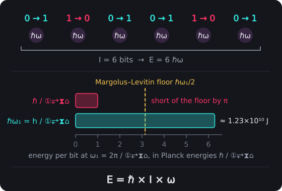
Information-Energy Equivalence. Each bit is one binary transition carrying one quantum ℏω, so I bits carry E = ℏ × I × ω. At ω₁ = 2π/①⥂⧗⌂ a bit carries h/①⥂⧗⌂ ≈ 1.23 × 10¹⁰ J, 2π Planck energies: twice the Margolus–Levitin floor ℏω₁/2, while the cycle-rate reading ℏ/①⥂⧗⌂ falls short of that floor by π.
UniSpheral Energy System Evolution G
S(n+1) = f[(n+1)²] × E⊶₁ [𝕄·𝕃²·𝕋⁻²]
Dimensional analysis:
Where (from the book): n [∅], ℏ [𝕄·𝕃²·𝕋⁻¹]
Read dimensionally: S(n+1) = f((n+1)²) × E⊶₁
[𝕄·𝕃²·𝕋⁻²]
[∅]([∅]) × [𝕄·𝕃²·𝕋⁻²] = [∅] × [𝕄·𝕃²·𝕋⁻²] = [𝕄·𝕃²·𝕋⁻²]
[𝕄·𝕃²·𝕋⁻²] = [𝕄·𝕃²·𝕋⁻²] ✓ Valid PulseCore Verified ✓
Level 2: Data Gravity (meso, recursive neighborhood coupling)
Where:
- S(n+1) [𝕄·𝕃²·𝕋⁻²] – system energy at next step
- f[] [∅] – threshold modulation function
- n [∅] – number of active neighboring states
- (n+1)² [∅] – quadratic neighborhood term
- E⊶₁ [𝕄·𝕃²·𝕋⁻²] – base transition energy = ℏ × ω₁
- ℏ [𝕄·𝕃²·𝕋⁻¹] – reduced Planck constant
- ω₁ [𝕋⁻¹] – fundamental frequency
➢ Neighborhood interactions compound quadratically, creating recursive density that manifests as gravitational attraction and curvature.
Data Energy Critical Threshold Condition G
Σ field_tension ≥ PD × τ⥂ × Θ⨶
Level 3: Collapse Threshold (macro, Null Well formation)
Where:
- Σ field_tension [𝕄·𝕃²·𝕋⁻²] – accumulated recursive tension
- PD [𝕃] – pulse diameter
- τ⥂ [𝕋] – pulse duration
- Θ⨶ [𝕄·𝕃·𝕋⁻³] – tolerance factor; the critical rate at which tension builds (force per unit time), so that a diameter crossed for one pulse duration holds exactly the threshold energy
- ≥ [∅] – inequality operator
- Σ [∅] – summation operator
➢ Once recursive density exceeds substrate capacity, local physical recursion appears to halt, forming a Null Well. This is gravity at its absolute maximum — not infinite curvature but a rupture. Seen from outside, physical evolution stops, as a clock appears to stop at an event horizon; the data does not stop, but turns onto the new dimension the rupture opens (Rupture Rule, Chapter 1, Part D.3).
Macroscopic collapse threshold where accumulated field tension exceeds critical substrate capacity, triggering Null Well formation through systematic breakdown of computational architecture when recursive density overwhelms fundamental pulse timing constraints.
Thus, what physics treats as separate domains — quantum energy levels, gravitational attraction, and cosmic collapse — are unified expressions of data recursion within the UniSphere. Data energy defines the quanta of existence, data gravity emerges from recursive amplification, and collapse thresholds determine when physical recursion falls still at a rupture. Together they form the computational architecture of the cosmos, where every constant, field, and structure is derivative of data’s recursive dynamics.
Recursive Data Energy Amplification Dynamics
In the UniSphere, energy evolution advances stepwise through recursive binary operations. Each computational increment does not simply add energy linearly but amplifies quadratically, since every state interacts with its neighbors. This creates local recursive coupling effects that scale the base transition energy into macroscopic outcomes. System energy is therefore not imposed externally but generated from within the lattice of the UniSphere itself, where recursive density and threshold modulation govern the amplification process (Strogatz, 1994).
The Base Calculation includes neighborhood interaction effects creating exponential amplification, similar to cooperative phenomena in critical systems (Wilson, 1971; Kadanoff, 2000).
The UniSpheral Energy System Evolution of Level 1, S(n+1) = f[(n+1)²] × E⊶₁ (above), amplifies by neighborhood:
➢ Neighborhood interactions create quadratic amplification effects, revealing how local computational interactions generate macroscopic energy phenomena (Strogatz, 1994).
Boundary Analysis: The function f[x] must satisfy stability conditions: f[x] = 1 for x < T⨶ (stable amplification), f[x] = 0 for x > T⨶ (collapse to null state), with continuity at threshold ensuring smooth transitions.
UniSpheral System energy emerges through quadratic neighborhood amplification, where recursive state coupling transforms microscopic transition quanta into macroscopic energetic structure. The modulation function f[] enforces collapse thresholds, ensuring that quadratic growth remains bounded. In this way, Binary Pulse Theory reframes energetic emergence as a computational inevitability: local recursive interactions compound into large-scale energy, with collapse thresholds maintaining balance between expansion and the apparent stillness of collapse.
Quantum Mechanical Correspondence
In the UniSphere, what appears in physics as quantum harmonic oscillator energy levels emerges directly from recursive binary transitions. The Base Calculation proposes that discrete spectra are not arbitrary impositions of quantum theory but natural outcomes of pulse discretization at Planck intervals. By aligning the computational substrate with oscillator dynamics, Binary Pulse Theory reproduces the canonical energy spectrum while exposing its underlying logic (Weinberg, 1995).
Quantum Energy Spectrum
E_n = ℏ × ω × (n + 1/2) [𝕄·𝕃²·𝕋⁻²]
Where:
- E_n [𝕄·𝕃²·𝕋⁻²] – Energy of quantum state n
- ℏ [𝕄·𝕃²·𝕋⁻¹] – Reduced Planck constant
- ω [𝕋⁻¹] – Angular frequency of quantum oscillator
- n [∅] – Quantum number (non-negative integer)
- 1/2 [∅] – Zero-point energy coefficient
Dimensional analysis:
Where (from the book): E_n [𝕄·𝕃²·𝕋⁻²], ℏ [𝕄·𝕃²·𝕋⁻¹], ω [𝕋⁻¹], n [∅], 1/2 [∅]
[𝕄·𝕃²·𝕋⁻²]
[𝕄·𝕃²·𝕋⁻¹] × [𝕋⁻¹] × ([∅] + [∅]) = [𝕄·𝕃²·𝕋⁻²] × ([∅] + [∅]) = [𝕄·𝕃²·𝕋⁻²] × [∅] = [𝕄·𝕃²·𝕋⁻²]
[𝕄·𝕃²·𝕋⁻²] = [𝕄·𝕃²·𝕋⁻²] ✓ Valid PulseCore Verified ✓
➢ Binary state transitions at ①⥂⧖ intervals reproduce the discrete energy spectrum of quantum harmonic oscillators, revealing the computational substrate underlying quantum mechanics.
Discrete energy quantization in harmonic oscillator systems where quantum states exhibit equal spacing with zero-point energy offset, establishing fundamental quantum mechanical energy levels that emerge from substrate oscillation frequencies through computational state discretization.
Thus, quantum mechanical energy quantization is not a mystery of wave–particle duality but a direct consequence of binary recursion at the substrate level. The zero-point offset reflects the irreducible presence of the Prime Pulse, while the evenly spaced spectrum arises from successive state increments in the UniSpheral lattice. In BPT, quantum mechanics is not fundamental but emergent from computation itself, unifying oscillator spectra, digital physics approaches (Fredkin, 2003; Wolfram, 2002), and Binary Pulse Theory into a single framework.
3.1 Testable Predictions
- Quantum Transition Timing: Energy transitions in quantum systems should exhibit temporal discretization at ①⥂⧖⌂ = ①⥂⧗⌂/2 intervals, detectable through ultra-high precision spectroscopy measurements with femtosecond temporal resolution.
- Neighborhood Amplification Effects: Phase transitions in condensed matter should demonstrate (n+1)² scaling relationships in critical exponents, verifiable through statistical analysis of cooperative transition dynamics (Wilson, 1971).
- Computational Energy Signatures: Information processing systems should exhibit measurable energy costs consistent with E⊶ = ℏ × ω₁ calculations, testable through precision calorimetry of quantum computational devices.
- Frequency Quantization: All physical processes should exhibit fundamental frequency relationships based on ω₁ = 2π/①⥂⧗⌂, detectable through high-resolution frequency analysis across multiple physical systems.
The Base Calculation indicates that what we call "physical energy" is actually computational energy — the Universe literally runs on information processing. BPT holds that this is not metaphor but physics that would be measurable: every quantum transition, every chemical reaction, every stellar fusion process operates through the binary computational substrate that Binary Pulse Theory proposes. On this view, reality is computation, and computation is energy generation.