Chapter 3 · Section 6
Data Novas and Dimensional Evolution
What if dimensions aren't given but created through computational overflow? When Data Nova calculations reach critical thresholds, computational transformation transcends energy release to trigger dimensional structure formation itself. Toroidal Genesis represents the first act of dimensional creation, where recursive Data Density crystallizes into computational geometry sustaining all subsequent reality, following conformal field theory principles (Polchinski, 1998).
The Breaking Point of the UniSphere: How Data Novas Ignite
A Data Nova is not a random eruption but the predictable outcome of recursive buildup. Each cycle of recursion increases structural capacity according to a simple quadratic law. When this growing capacity surpasses the system’s allowable threshold, stability can no longer be maintained, and recursion is forced to reorganize into a higher-dimensional framework. This crossing point is the true ignition of a Data Nova — the computational boundary where recursive growth transforms into creation.
The UniSpheral Data Nova Threshold Law G
The UniSpheral Nova Threshold Law defines when recursion must erupt into a Data Nova.
It occurs when quadratic capacity growth f(n) overwhelms the containment threshold χ_∂, the holographic capacity of the containing skin (the Bifold Containment Law, below).
At this exact step n*, the Pulsecore reorganizes into higher-dimensional structure.
Recursive Capacity Growth G
f(n) = (n + 1)² [∅]
Dimensional analysis:
[∅]([∅]) = [∅]
([∅] + [∅])² = [∅]² = [∅]
[∅] = [∅] ✓ Valid PulseCore Verified ✓
Shows how recursive depth expands structural capacity quadratically with each step.
Containment Crossing Condition G
n* = ceil(√(χ_∂) - 1) [∅]
Dimensional analysis:
Where (from the book): 1 [∅], f(n) [∅], n [∅], n* [∅], χ_∂ [∅], ceil [∅], √ [∅]
[∅]
[∅]([∅]([∅]) - [∅]) = [∅]([∅] - [∅]) = [∅]([∅]) = [∅]
[∅] = [∅] ✓ Valid PulseCore Verified ✓
Defines the minimum recursion depth where capacity first overwhelms the toroidal threshold, forcing reorganization.
Where:
- f(n) [∅] – structural capacity after n recursive steps
- n [∅] – recursion step
- n* [∅] – minimum recursion step for the Data Nova
- χ_∂ [∅] – containment threshold in capacity units: the holographic capacity of the containing skin (Bifold Containment Law)
- ceil [∅] – ceiling function
- √ [∅] – square root function
- 1 [∅] – unity offset constant
➢ The Data Nova occurs when accumulated recursive capacity f(n) reaches the containment threshold χ_∂, requiring system reorganization into higher-dimensional structure. The Null Nova comes before it, at half that capacity, when the data and its null fill the boundary together (the Null Nova Condition, below).
The threshold n* = ceil(√(χ_∂) - 1) provides a precise computational step where dimensional reorganization becomes inevitable, following principles from Rovelli's quantum gravity framework (Rovelli, 2004).
Together, these two expressions form the UniSpheral Nova Threshold Law. The first equation maps the natural growth of recursion, while the second pinpoints the exact computational step at which a Data Nova must occur. In practice, f(n) describes the fuel, χ_∂ the container (the skin), and n* the match that lights the transformation.
This framework holds that Data Novas are lawful, predictable events — not explosions out of chaos but phase transitions built into the UniSphere’s computational code, consistent with Rovelli’s approaches to quantum gravity.
The Pulsecore as a Bubble of Data
What is the Pulsecore doing while it fills toward its novas? A universe begins across three parts. On the parent's side is the Nullcore, the singularity at the bottom of a null well, where the parent's data sinks to 0. Between them is the Bifold, the line between the dimensions, the one fold where one universe becomes two (the Prime Pulse bifurcation ∅ → (0 ↔ 1)). On the child's side is the Pulsecore, the child's data held within the Bifold: the binary pulse written across the boundary, 0 | 1. The Pulsecore is a bubble, and the Bifold is its skin. It is Planck-sized in the units of the universe it begins, and it holds data inside as well as on its surface. Before the physical layer (Temporal Genesis, below) that data has no mass, since mass belongs to the physical, so nothing holds it back. It is not a gas, which is matter with mass and collisions of its own, but radiation: it moves freely at the local light speed 𝒞→ and fills the Pulsecore as light fills a hot cavity. The data within crosses the bubble, strikes the Bifold, is written there and sent back in, and turns with the spin of the Bifold that holds it. Every bit carries its null, the 0 of its own pulse, so the Pulsecore holds its null as well as its data, and the Bifold holds as long as it can record what it contains. It gives way twice: first to the null, at the Null Nova, which becomes space, and then to the data, at the Data Nova, which pours out onto that space. Six laws describe it, and the fourth gives the Nova Threshold Law's containment threshold its meaning. When the novas have emptied it, the Pulsecore is the Nullcore again, seen from inside: the Nullcore and the child's emptied core are one vacuum, the Null Vacuum of Part 3.13.
Pulsecore Data Radiance G
P_∂ = u / 3 [𝕄·𝕃⁻¹·𝕋⁻²]
Dimensional analysis:
Where (from the book): 3 [∅], P_∂ [𝕄·𝕃⁻¹·𝕋⁻²], u [𝕄·𝕃⁻¹·𝕋⁻²], n [𝕃⁻³], T [Θ], v [𝕃·𝕋⁻¹]
[𝕄·𝕃⁻¹·𝕋⁻²]
[𝕄·𝕃⁻¹·𝕋⁻²] ÷ [∅] = [𝕄·𝕃⁻¹·𝕋⁻²]
[𝕄·𝕃⁻¹·𝕋⁻²] = [𝕄·𝕃⁻¹·𝕋⁻²] ✓ Valid PulseCore Verified ✓
u = n · k_B · T [𝕄·𝕃⁻¹·𝕋⁻²]
Dimensional analysis:
Where (from the book): 3 [∅], P_∂ [𝕄·𝕃⁻¹·𝕋⁻²], u [𝕄·𝕃⁻¹·𝕋⁻²], n [𝕃⁻³], T [Θ], v [𝕃·𝕋⁻¹]
[𝕄·𝕃⁻¹·𝕋⁻²]
[𝕃⁻³] × [𝕄·𝕃²·𝕋⁻²·Θ⁻¹] × [Θ] = [𝕄·𝕃⁻¹·𝕋⁻²·Θ⁻¹] × [Θ] = [𝕄·𝕃⁻¹·𝕋⁻²]
[𝕄·𝕃⁻¹·𝕋⁻²] = [𝕄·𝕃⁻¹·𝕋⁻²] ✓ Valid PulseCore Verified ✓
v = 𝒞→ [𝕃·𝕋⁻¹]
Dimensional analysis:
Where (from the book): 3 [∅], P_∂ [𝕄·𝕃⁻¹·𝕋⁻²], u [𝕄·𝕃⁻¹·𝕋⁻²], n [𝕃⁻³], T [Θ], v [𝕃·𝕋⁻¹]
[𝕃·𝕋⁻¹]
[𝕃·𝕋⁻¹]
[𝕃·𝕋⁻¹] = [𝕃·𝕋⁻¹] ✓ Valid PulseCore Verified ✓
Massless data within the Pulsecore is radiation, not a gas: every datum moves at the local light speed, and its pressure is a third of its energy density.
Where:
- P_∂ [𝕄·𝕃⁻¹·𝕋⁻²] – pressure of the data within on the skin
- u [𝕄·𝕃⁻¹·𝕋⁻²] – energy density of the data within
- n [𝕃⁻³] – number density of data within
- k_B [𝕄·𝕃²·𝕋⁻²·Θ⁻¹] – Boltzmann constant, the one constant every universe shares
- T [Θ] – the Pulsecore's temperature
- v [𝕃·𝕋⁻¹] – a datum's speed
- 𝒞→ [𝕃·𝕋⁻¹] – the local light speed, Length / Tempo
- 3 [∅] – the three directions a datum may move in
➢ Each datum carries the Data Energy E = k_B·T of one substrate pulse (Part 1), so the energy density is the number density times k_B·T. For anything that moves at light speed, the pressure is a third of the energy density, the law of radiation in a cavity, which physics calls a photon gas only by analogy (Planck, 1901; Tolman, 1934). Heat raises the pressure and never the speed: a datum within the Pulsecore is always at 𝒞→, and only its direction changes, at each strike of the skin. This is why the Pulsecore glows as a heated body does as it fills. Radiation squeezed does not stack up as matter does: each datum that strikes an inward-moving wall returns with more energy, so compressing it slowly keeps its count and raises its temperature as T ∝ V^(−1/3), its energy density as T⁴. Light is made of bosons, which share a state without limit, as a laser's photons do, unlike the electrons of matter, which exclude one another (Pauli, 1925; Bose, 1924). Nothing in the radiation itself stops it being packed tighter; what caps it is the information its boundary can record, which grows with the boundary's area (Bekenstein, 1973). That is the Bifold's limit: a limit on records, not on room.
Bifold Record Law G
Φ_∂ = n · 𝒞→ / 4 [𝕃⁻²·𝕋⁻¹]
Dimensional analysis:
Where (from the book): 4 [∅], Φ_∂ [𝕃⁻²·𝕋⁻¹], n [𝕃⁻³]
[𝕃⁻²·𝕋⁻¹]
[𝕃⁻³] × [𝕃·𝕋⁻¹] ÷ [∅] = [𝕃⁻²·𝕋⁻¹] ÷ [∅] = [𝕃⁻²·𝕋⁻¹]
[𝕃⁻²·𝕋⁻¹] = [𝕃⁻²·𝕋⁻¹] ✓ Valid PulseCore Verified ✓
The Bifold is the record of the data within: every datum that strikes it is written where it strikes, and the skin sends data back in.
Where:
- Φ_∂ [𝕃⁻²·𝕋⁻¹] – strikes on the skin per unit area per unit time
- n [𝕃⁻³] – number density of data within
- 𝒞→ [𝕃·𝕋⁻¹] – the local light speed
- 4 [∅] – the kinetic factor for data moving in every direction at one speed
➢ For data moving in all directions at one speed, a quarter of n·𝒞→ crosses each unit of the wall each unit of time, the flux of kinetic theory. The skin is where the interior becomes visible: what we see on the Pulsecore's surface is the record of what has struck it, as the holographic principle reads a horizon as the record of what lies within it ('t Hooft, 1993; Susskind, 1995; Bousso, 2002). The skin is as hot as the data it holds, and it returns data at the Pulsecore's temperature, the thermal wall of kinetic theory. So the patterns on a Pulsecore's surface are made by its interior, and are not separate from it.
Bifold Drag G
v_∂ = 𝒞→ · a_f / (1 + √(1 − a_f²)) [𝕃·𝕋⁻¹]
Dimensional analysis:
Where (from the book): v_∂ [𝕃·𝕋⁻¹], n(ρ) [𝕃⁻³], n₀ [𝕃⁻³], γ(ρ) [∅], Ω [𝕋⁻¹], ρ [𝕃]
[𝕃·𝕋⁻¹]
[𝕃·𝕋⁻¹] × [∅] ÷ ([∅] + √([∅] - [∅])) = [𝕃·𝕋⁻¹] ÷ ([∅] + √([∅] - [∅])) = [𝕃·𝕋⁻¹] ÷ ([∅] + √[∅]) = [𝕃·𝕋⁻¹] ÷ ([∅] + [∅]) = [𝕃·𝕋⁻¹] ÷ [∅] = [𝕃·𝕋⁻¹]
[𝕃·𝕋⁻¹] = [𝕃·𝕋⁻¹] ✓ Valid PulseCore Verified ✓
n(ρ) = n₀ · γ(ρ)³ [𝕃⁻³]
Dimensional analysis:
Where (from the book): v_∂ [𝕃·𝕋⁻¹], n(ρ) [𝕃⁻³], n₀ [𝕃⁻³], γ(ρ) [∅], Ω [𝕋⁻¹], ρ [𝕃]
[𝕃⁻³]
[𝕃⁻³] × [∅] = [𝕃⁻³]
[𝕃⁻³] = [𝕃⁻³] ✓ Valid PulseCore Verified ✓
The Bifold turns with the universe's spin, its equator at the speed of a spinning horizon's equator, and drags the data it touches, so the data within swirls with the spin and crowds toward the equator.
Where:
- v_∂ [𝕃·𝕋⁻¹] – speed of the skin at its equator
- a_f [∅] – the universe's dimensionless spin, 0 ≤ a_f < 1
- 𝒞→ [𝕃·𝕋⁻¹] – the local light speed
- n(ρ) [𝕃⁻³] – density of data within at distance ρ from the spin axis
- n₀ [𝕃⁻³] – density of data within on the spin axis
- γ(ρ) [∅] – 1 / √(1 − Ω²ρ²/𝒞→²), the Lorentz factor of the co-rotating data at ρ
- Ω [𝕋⁻¹] – the skin's angular velocity
- ρ [𝕃] – distance from the spin axis
➢ The skin's equator moves as the equator of a Kerr horizon does: the horizon's angular velocity times its equatorial circumference radius gives a_f / (1 + √(1 − a_f²)) of light speed. That is 0 for a spinless Pulsecore and approaches light speed as the spin approaches its limit, never reaching it (Kerr, 1963; Bardeen, Press & Teukolsky, 1972). A datum that strikes a turning wall leaves it carrying the wall's motion along the surface, so the spinning skin drags the data within, as a turning container spins up what it holds. In equilibrium, co-rotating radiation is hotter, and so denser, away from the axis, its temperature rising with the Lorentz factor of its motion (Tolman, 1934). The data gathers toward the equator, the band the Data Nova throws outward.
Bifold Containment Law G
P_∂ ≤ 2 · σ_∂ / R [𝕄·𝕃⁻¹·𝕋⁻²]
Dimensional analysis:
Where (from the book): P_∂ [𝕄·𝕃⁻¹·𝕋⁻²], σ_∂ [𝕄·𝕋⁻²], R [𝕃], A [𝕃²], χ_∂ [∅], N [∅], T [Θ], 2, [∅]
[𝕄·𝕃⁻¹·𝕋⁻²] ≤ [∅] × [𝕄·𝕋⁻²] ÷ [𝕃] = [𝕄·𝕃⁻¹·𝕋⁻²] ≤ [𝕄·𝕋⁻²] ÷ [𝕃] = [𝕄·𝕃⁻¹·𝕋⁻²] ≤ [𝕄·𝕃⁻¹·𝕋⁻²] ✓ Valid PulseCore Verified ✓
χ_∂ = A / (4 · ln(2) · ℓ_p²) · ℨᵇ [1ᵇ]
Dimensional analysis:
Where (from the book): P_∂ [𝕄·𝕃⁻¹·𝕋⁻²], σ_∂ [𝕄·𝕋⁻²], R [𝕃], A [𝕃²], χ_∂ [1ᵇ], N [1ᵇ], T [Θ], 2, [∅]
[1ᵇ]
[𝕃²] ÷ ([∅] × [∅] × [𝕃²]) × [1ᵇ] = [𝕃²] ÷ ([∅] × [𝕃²]) × [1ᵇ] = [𝕃²] ÷ [𝕃²] × [1ᵇ] = [∅] × [1ᵇ] = [1ᵇ]
[1ᵇ] = [1ᵇ] ✓ Valid PulseCore Verified ✓
σ_∂ = k_B · T / (8 · ln(2) · ℓ_p²) [𝕄·𝕋⁻²]
Dimensional analysis:
Where (from the book): P_∂ [𝕄·𝕃⁻¹·𝕋⁻²], σ_∂ [𝕄·𝕋⁻²], R [𝕃], A [𝕃²], χ_∂ [∅], N [∅], T [Θ], 2, [∅]
[𝕄·𝕋⁻²]
[𝕄·𝕃²·𝕋⁻²·Θ⁻¹] × [Θ] ÷ ([∅] × [∅] × [𝕃²]) = [𝕄·𝕃²·𝕋⁻²] ÷ ([∅] × [∅] × [𝕃²]) = [𝕄·𝕃²·𝕋⁻²] ÷ ([∅] × [𝕃²]) = [𝕄·𝕃²·𝕋⁻²] ÷ [𝕃²] = [𝕄·𝕋⁻²]
[𝕄·𝕋⁻²] = [𝕄·𝕋⁻²] ✓ Valid PulseCore Verified ✓
N ≥ χ_∂ [1ᵇ]
Dimensional analysis:
Where (from the book): P_∂ [𝕄·𝕃⁻¹·𝕋⁻²], σ_∂ [𝕄·𝕋⁻²], R [𝕃], A [𝕃²], χ_∂ [1ᵇ], N [1ᵇ], T [Θ], 2, [∅]
[1ᵇ] ≥ [1ᵇ] ✓ Valid PulseCore Verified ✓
The Pulsecore holds while the Bifold can record what it contains; when the data within fills the skin's holographic capacity, N ≥ χ_∂, the bubble bursts, and that is the Data Nova.
Where:
- P_∂ [𝕄·𝕃⁻¹·𝕋⁻²] – pressure of the data within (Pulsecore Data Radiance)
- σ_∂ [𝕄·𝕋⁻²] – tension of the skin, the dimensional boundary tension σ◫ of Part 4.3 for the Bifold
- R [𝕃] – radius of the Pulsecore
- A [𝕃²] – area of the skin, 4πR²
- χ_∂ [1ᵇ] – the skin's holographic capacity in Zinf bits: the containment threshold
- N [1ᵇ] – the data within, in Zinf bits
- ℨᵇ [1ᵇ] – one Zinf bit, the unit a capacity made from areas is counted in
- ℓ_p [𝕃] – the local Planck length of the universe the Pulsecore begins
- k_B [𝕄·𝕃²·𝕋⁻²·Θ⁻¹] – Boltzmann constant
- T [Θ] – the Pulsecore's temperature
- ln2 [∅] – natural logarithm of 2, nats to bits
- 2, 4, 8 [∅] – geometric factors
➢ The book's Containment Force Balance (Part 4.3) sets the skin's tension over its area against the internal pressure through its volume, F = σA − PV. A bubble stands where that balance is stationary in its radius, 8πRσ = 4πR²P, which is Laplace's law of a bubble, P = 2σ/R (Young, 1805; Laplace, 1806). The skin's capacity is its horizon count, one bit for every 4·ln2 Planck areas (Bekenstein, 1973; Hawking, 1975). With the data's pressure P = N·k_B·T / (3V), the two conditions are one when the skin's tension is σ_∂ = k_B·T / (8·ln2·ℓ_p²): then the temperature cancels, and the bubble bursts exactly when N reaches χ_∂, whatever its heat. The skin's tension rises with its temperature as the data's pressure does, so heating the Pulsecore brings it no nearer the burst; only more data does. That is why the Data Nova comes at a definite count, as the Nova Threshold Law says it must.
This is the containment threshold of the Nova Threshold Law: χ_∂ is the holographic capacity of the skin that contains the data, the Bifold for the Pulsecore's two Novas and the torus's for each Nova after it. The Bifold records every state within, the 0 as well as the 1: before the Null Nova it holds the data and their null, after it the data alone. The quadratic growth f(n) = (n + 1)² grows as an area does, which is what a skin's record does. At the Data Nova the bubble turns inside out (Part 3.7). The Pulsecore, emptied first of its null and then of its data, holds neither: it becomes the Null Vacuum, a true vacuum, the hole the torus circulates through: the same vacuum as the Nullcore at the bottom of the parent's well, and the space whose Vacuum Pressure drives the late expansion (Part 3.13).
Null Nova Condition G
N_∅ = N [1ᵇ]
Dimensional analysis:
Where (from the book): N [1ᵇ], N_∅ [1ᵇ], ρ_∅ [∅], χ_∂ [1ᵇ], N₁ [1ᵇ], n₁ [∅], ceil, [∅]
[1ᵇ]
[1ᵇ]
[1ᵇ] = [1ᵇ] ✓ Valid PulseCore Verified ✓
ρ_∅ = N / (χ_∂ − N) [∅]
Dimensional analysis:
Where (from the book): N [1ᵇ], N_∅ [1ᵇ], ρ_∅ [∅], χ_∂ [1ᵇ], N₁ [1ᵇ], n₁ [∅], ceil, [∅]
[∅]
[1ᵇ] ÷ ([1ᵇ] - [1ᵇ]) = [1ᵇ] ÷ [1ᵇ] = [∅]
[∅] = [∅] ✓ Valid PulseCore Verified ✓
N + N_∅ = χ_∂ [1ᵇ]
Dimensional analysis:
Where (from the book): N [1ᵇ], N_∅ [1ᵇ], ρ_∅ [∅], χ_∂ [1ᵇ], N₁ [1ᵇ], n₁ [∅], ceil, [∅]
[1ᵇ] + [1ᵇ] = [1ᵇ]
[1ᵇ]
[1ᵇ] = [1ᵇ] ✓ Valid PulseCore Verified ✓
N₁ = χ_∂ / 2 [1ᵇ]
Dimensional analysis:
Where (from the book): N [1ᵇ], N_∅ [1ᵇ], ρ_∅ [∅], χ_∂ [1ᵇ], N₁ [1ᵇ], n₁ [∅], ceil, [∅]
[1ᵇ]
[1ᵇ] ÷ [∅] = [1ᵇ]
[1ᵇ] = [1ᵇ] ✓ Valid PulseCore Verified ✓
n₁ = ceil(√(χ_∂ / (2 · ℨᵇ)) − 1) [∅]
Dimensional analysis:
Where (from the book): N [1ᵇ], N_∅ [1ᵇ], ρ_∅ [∅], χ_∂ [1ᵇ], N₁ [1ᵇ], n₁ [∅], ceil, [∅]
[∅]
ceil(√([1ᵇ] ÷ ([∅] × [1ᵇ])) - [∅]) = ceil(√([1ᵇ] ÷ [1ᵇ]) - [∅]) = ceil(√[∅] - [∅]) = ceil([∅] - [∅]) = ceil([∅]) = [∅]
[∅] = [∅] ✓ Valid PulseCore Verified ✓
Every bit carries its null; packed into the room the data has not taken, the null grows denser until data and null together fill the Bifold's record, and the Pulsecore gives its null up as space.
Where:
- N [1ᵇ] – the data within, in Zinf bits, f(n) = (n + 1)² after n Tempos
- N_∅ [1ᵇ] – the null within: the 0 of each bit's pulse, one for every bit
- ρ_∅ [∅] – the null's density: nulls per place the data has not taken
- χ_∂ [1ᵇ] – the Bifold's holographic capacity, 16·4^L Zinf bits at level L (Bifold Containment Law)
- N₁ [1ᵇ] – the data within at the Null Nova
- ℨᵇ [1ᵇ] – one Zinf bit; χ_∂ / ℨᵇ is the capacity as a number
- n₁ [∅] – the Tempo of the Null Nova
- ceil, √, 1, 2 [∅] – ceiling, square root, unity offset and the two states of a pulse
➢ A pulse is 0 → 1 → 0: each bit is the 1 of a pulse whose 0 comes with it, so a Pulsecore that holds N bits holds N nulls. A place records one state a Rhythm, a 1 or a 0 (the UniSpheral Data Information Capacity, Chapter 1), so the null needs room as the data does. Before any space exists there is nowhere else for it to go, and it is packed into the places the data has not taken, ρ_∅ = N / (χ_∂ − N), rising from nothing toward one. When it reaches one, the data and its null fill the Bifold's record together, N = χ_∂ / 2, and the Bifold gives way to what it holds least: the null, which carries no bit and so no record, leaves, while the data, written in the Bifold's record, stays. The data's count bursts the Bifold; what leaves first is the null. The null leaving is space: the empty toroidal form, the first layer (Toroidal Genesis, below). The order is the order of logic, since a bit is written into a place and the places come before the bits that fill them, and standard cosmology keeps the same order: inflation stretches space nearly empty, driven by the energy of the vacuum, before reheating fills it with radiation and particles (Guth, 1981; Kofman, Linde & Starobinsky, 1994).
Space Growth Law G
S(n) = N(n) = (n + 1)² · ℨᵇ [1ᵇ]
Dimensional analysis:
Where (from the book): S(n) [1ᵇ], N(n) [1ᵇ], n [∅], χ_∂ [1ᵇ]
[1ᵇ]
[1ᵇ]
([∅] + [∅])² × [1ᵇ] = [∅]² × [1ᵇ] = [∅] × [1ᵇ] = [1ᵇ]
[1ᵇ] = [1ᵇ] = [1ᵇ] ✓ Valid PulseCore Verified ✓
χ_∂ / 2 ≤ S(n) ≤ χ_∂ [1ᵇ]
Dimensional analysis:
Where (from the book): S(n) [1ᵇ], N(n) [1ᵇ], n [∅], χ_∂ [1ᵇ]
[1ᵇ] ÷ [∅] ≤ [1ᵇ] ≤ [1ᵇ] = [1ᵇ] ≤ [1ᵇ] ≤ [1ᵇ] ✓ Valid PulseCore Verified ✓
After the Null Nova each new bit's null leaves as it is made, so space grows one place for every bit, and at the Data Nova it holds exactly one place for every bit waiting in the Pulsecore.
Where:
- S(n) [1ᵇ] – the places of space after n Tempos, from the Null Nova to the Data Nova, one Zinf bit of room each
- N(n) [1ᵇ] – the data within after n Tempos, in Zinf bits
- ℨᵇ [1ᵇ] – one Zinf bit
- n [∅] – Tempos since the Pulsecore was sealed
- χ_∂ [1ᵇ] – the Bifold's holographic capacity
➢ Once the Null Nova has made an outside, the null of each new bit leaves for it as soon as it is made: space grows by one place for every bit, from χ_∂ / 2 places at the Null Nova to χ_∂ at the Data Nova, its area doubling. Only the data still presses on the Bifold, so the Pulsecore goes on filling with bits alone until they fill the record, N ≥ χ_∂ (χ_∂ = (4·2^L)² is a perfect square, so the count meets it exactly), at n₂ = ceil(√χ_∂ − 1) = 4·2^L − 1 Tempos: the Data Nova (the Nova Threshold Law above). Then the data pours out onto space that holds exactly χ_∂ places, one for every bit, so a universe's field is built to the size of its data before its data arrives, with nothing tuned to make it so; this count is the Local Pixel Count, 16·4^L (Chapter 1). At level 1 the Null Nova comes at Tempo 5 and the Data Nova at Tempo 7; at level 6, at Tempos 181 and 255.
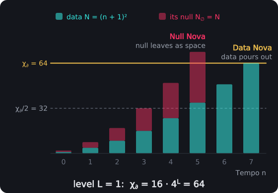
The Pulsecore Fills Toward Its Novas. At level 1 the Bifold holds χ∂ = 16 · 4¹ = 64 bits. The data N = (n + 1)² and its null fill it together at Tempo 5, N = χ∂/2, and the null leaves as space: the Null Nova. The data alone reaches χ∂ at Tempo 7: the Data Nova.
The Null Nova and Toroidal Genesis
Dimensional expansion for a new universe begins not with a random blast but with a precise computational Pulse — the Null Nova, the Pulsecore's first. When the data within, f(n) = (n + 1)² by the Recursive Capacity Law, and its null together fill the Bifold's record (the Null Nova Condition), the null does not scatter or explode chaotically in this phase, as in a Big Bang. Instead, it reorganizes into a closed-loop Toroidal Substrate, the first computational geometry of a universe, like an ethereal prime layer. This torus becomes the processor of a newborn domain, sustaining the Prime Pulse bifurcation ∅ → (0 ↔ 1) and locking recursion into stable continuity.
Unlike conventional Big Bang cosmology that imagines expansion radiating from a singular point (Hawking, 1975; Guth, 1981), the Null Nova crystallizes a self-contained geometry. The torus folds boundary into motion, ensuring continuity between inside and outside. Information is not lost but continuously recirculated, consistent with Penrose’s conformal boundary framework (Penrose, 2005).
The torus is not incidental — it is computation’s first act. Its looping form encodes recursion and memory into geometry, making the Null Nova the genesis not of matter but of the architecture that carries matter into being, echoing Wheeler’s “it from bit” hypothesis (Wheeler, 1989).
Escalation and Physical Reality Through Successive Data Novas
Creation of a Physical Universe does not occur in a single act but through a sequence of distinct computational discharges — each one a Data Event with its own outcome. The first Data Event, the Null Nova, is the ignition of the Toroidal Pulse itself. It does not create matter or dimension but forges the toroidal substrate, the closed-loop architecture capable of sustaining recursion. The Null Nova is the genesis of architecture: a geometry that encodes memory and continuity, ensuring that binary transitions ∅ → (0 ↔ 1) do not vanish but cycle.
Dimensional growth occurs in punctuated surges through Data Nova Escalation, each triggered when recursive Data Density exceeds toroidal containment. Rather than infinite smooth expansion, Binary Pulse Theory posits stepwise dimensional ladders:
- First Nova (n=1), the Null Nova: Establishes toroidal genesis; the computational substrate itself, space without data, and the space that remains when the universe has gone (Part 3.10, After the Final Well).
- Second Nova (n=2), the Pulsecore's Data Nova: The data pours out onto the toroidal substrate and lays its lattice — first true expansion of data beyond containment, corresponding to new geometric axes (Weinberg, 2008).
- Third Nova (n=3), the Physical Nova: The big bang. Temporal stabilization emerges. Directional flow imposed upon recursive cycles, crystallizing causality — sewing time into space where symmetry gives way to irreversible direction (Greene, 1999).
- Fourth Nova (n=4), the Saturation Nova: Dimensional Saturation Threshold achieved. Three spatial and one temporal dimension cohere into a stable four-dimensional scaffold. Beyond this, Novas intensify harmonics but no longer create dimensional axes.
These stages suggest dimensionality itself is quantized — not infinite but discretely layered, with each Data Nova representing phase transition, echoing cosmological natural selection models where Universes trial different structural modes until stability is achieved (Smolin, 2013).
The UniSpheral Outward Expansion Set G
The UniSpheral Outward Expansion Set is the sequence of four Data Novas that transform recursion into physical reality. The process begins with Toroidal Genesis, the Null Nova, which forges the substrate architecture as empty space, followed by Dimensional Genesis, the Data Nova, where the data pours onto space and gives it its axes. Temporal Genesis then imposes the arrow of time, and Spacetime Genesis locks three spatial and one temporal axis into a stable 4D scaffold. Together, these punctuated surges show that universes emerge not in a single act, but through quantized phase transitions encoded in the UniSphere.
Toroidal Genesis G
(n = 1) The Null Nova
The first event, the Null Nova, is the ignition of the Toroidal Pulse itself: the null of the Pulsecore's bits expelled as space. It does not create matter or dimension but forges the toroidal substrate, empty of data, — the closed-loop computational geometry that encodes memory and recursion. Here, the Prime Pulse ∅ → (0 ↔ 1) is no longer a fleeting toggle but sustained as a cycling architecture, ensuring that recursion can persist. This is the genesis of architecture, the substrate processor upon which all further complexity depends.
Dimensional Genesis G
(n = 2) The Data Nova
The second event, the Data Nova (the Dimensional Nova), marks the first true expansion of data beyond containment: the Pulsecore's data pours out onto the space the Null Nova made and lays its lattice over it, generating new independent geometric axes. Space stood empty before; here it is first measured, its dimensionality the lattice of the data that fills it. This is the moment where spatial dimensionality first emerges: the raw scaffold of space itself. What arises is not yet matter, but the measurable axes that will later host energy, particles, and fields. With data on space comes the first place for collapse, and the first wells form here as data wells: regions where data falls in and is held, already part of the universe's census and already holding the information that will seed a child, but not yet physical. A data well sends no pulse into its surroundings and cannot orbit another, because both are events in time, and the time they need has not yet been laid down. Physics allows a well made of massless content: energy concentrated tightly enough curves spacetime into a horizon whatever carries it, and a black hole formed from light alone, a kugelblitz, follows from Wheeler's study of self-gravitating light (Wheeler, 1955). In our universe light focused toward that density is drained first by the pairs of matter it makes from the vacuum (the Schwinger effect), so no kugelblitz is expected to form from light today (Álvarez-Domínguez, Garay, Martín-Martínez & Polo-Gómez, 2024). Before the physical layer that drain has nowhere to go, since there is no matter yet for the data to become, and a well of pure data can form: a data well. The Dimensional Nova transforms recursion into geometry, creating the first framework of extension in the UniSphere.
Temporal Genesis G
(n = 3) Arrow of Time
The third event, the Causal Nova, imposes directionality upon recursion. Temporal stabilization emerges as symmetry breaks, sewing time into space and enforcing irreversibility. Causality crystallizes here: cycles no longer oscillate in perfect reversibility but gain an orientation, giving rise to ordered sequence and history. This nova is the genesis of the arrow of time, binding temporal flow to spatial structure.
Temporal Genesis is the physical layer. Data runs at the Pulse Rhythm, each single transition, while the physical runs at the Pulse Tempo, the full cycle that returns a state to itself, and a full cycle needs the arrow of time this nova lays down. It is the nova the simulation, and Parts 2.9 and 3.11, also call the Physical Nova. From the Data Nova until it, the data roams the scaffold freely, at light speed, filling the lattice; as the Causal Nova nears, the scaffold with all its data draws in to the pin head, the Pulsecore's own size, and then erupts as the physical universe, every part of it at once (Part 3.11). The physical layer is condensed from the data where it lies on the lattice, so the web of matter that grows from it traces the scaffold, as the visible web of galaxies in our universe traces the dark matter beneath it; and the data layer runs on beneath the physical, at the Pulse Rhythm, for the rest of the universe's life. Data comes before the arrow, not before the beat: from the Prime Pulse it keeps the Pulse Rhythm, each single transition, but until this nova its cycles are reversible, with no forward and no back, so data has rhythm without an arrow, and time as an order of events is built upon it here. Physics shows the same step from light to matter directly: two photons that collide with enough energy become an electron and a positron (Breit & Wheeler, 1934), and matter made from the collision of light alone has been measured (STAR Collaboration, 2021). So at the Causal Nova the data wells of the space layer become physical wells: they begin to pulse into the field around them, to orbit and to merge, and every well that forms from now on (Null Well Collapse, Part 3.9) is physical from its birth. A universe that ends before this layer, possible only at the shallowest levels, closes with data wells alone, and each still seeds its child, since a well's information is its child's Pulsecore whether or not it ever became physical.
Spacetime Genesis G
(n = 4) Four-Dimensional Scaffold
The fourth event, the Saturation Nova, achieves the Dimensional Saturation Threshold. At this stage, three spatial axes and one temporal axis cohere into a stable four-dimensional lattice — the spacetime fabric that underlies our universe. Beyond this point, further Novas do not generate new dimensions but instead intensify harmonic structure and resonance. These higher surges refine rather than expand, ensuring stability of the four-dimensional framework.
The UniSpheral Outward Expansion Set shows that the universe’s foundation is not the product of a singular detonation, but of a structured sequence of computational discharges. Each Data Nova marks a threshold where recursion is forced into new form, from the toroidal substrate to the dimensional scaffold of spacetime itself. By revealing creation as a ladder of quantized surges, Binary Pulse Theory reframes the origin of reality: physical existence is the outcome of ordered, recursive transitions within the UniSphere, not a random eruption from nothingness.
Dimensional Saturation and the Fourfold Limit
Recursive surges do not generate dimensions without end. Although the Recursive Capacity Law, f(n) = (n + 1)², describes unlimited algebraic growth, the Toroidal Substrate imposes strict geometric limits on how many independent axes can be supported.
Dimensional Saturation is the critical boundary where further recursive discharges no longer open new degrees of freedom but instead reinforce the lattice that already exists. This is the UniSpheral fourfold limit: the point where creation ceases to expand and begins to stabilize.
UniSpheral Dimensional Count Law G
D(n) = ∑ H(ΔI_i - I◉) [∅]
Where:
- D(n) [∅] – dimensional count at recursion level n
- ∑ [∅] – summation operator
- H [∅] – Heaviside step function
- ΔI_i [∅] – information increment at level i
- I◉ [∅] – substrate information capacity threshold
- i [∅] – summation index variable
- n [∅] – recursion level parameter
Dimensional analysis:
Where (from the book): ∑ [∅], H [∅], ΔI_i [∅], I◉ [∅], i [∅], n [∅]
Read dimensionally: D(n) = H(ΔI_i - I◉)
[∅]
[∅]([∅] - [∅]) = [∅]([∅]) = [∅]
[∅] = [∅] ✓ Valid PulseCore Verified ✓
➢ When D(n) approaches D⥣, expansion halts. The Universe locks into dimensional homeostasis — observed at our depth as three spatial dimensions braided with one temporal arrow. What sets D⥣ is a binding rule the theory has not yet fixed; it is not a cap of four.
Beyond this point, Data Novas shift function — from architects of new dimensions to custodians of harmony. They stabilize rather than expand, mirroring biological developmental saturation where organisms grow until stable form is reached (Kauffman, 1995).
When D(n) reaches D⥣, dimensional expansion halts. The UniSphere locks into its canonical framework — observed at our depth as three spatial dimensions braided with one temporal arrow. Beyond this threshold, Data Novas shift their role — no longer architects of new dimensional axes, they become custodians of harmony, refining resonance and stabilizing the scaffold.
Just as biological organisms grow until form reaches equilibrium, universes grow dimensionally until they reach a stable lattice, fourfold in ours. In Binary Pulse Theory, the four Data Novas offer a sequence by which this four-dimensional homeostasis forms; why recursive escalation stops at three spatial axes and one temporal axis at our depth is an open question the theory has not yet settled, since the binding rule that sets D⥣ is not yet fixed. Part 4.8 reads D⥣ as the prime limit of a universe's harmonics, the primes 2, 3, 5 and 7 for ours, and Part 3.13 finds that our sky's dark matter measures it: four.
Harmonic Reinforcement and Post-Saturation Novas
When the UniSphere reaches the Dimensional Saturation Threshold, further Data Novas do not vanish but transform in function. Post-saturation Novas are Harmonic Novas: discharges of recursive density that no longer create new axes but instead reinforce alignment within the existing four-dimensional lattice. By Data Harmonics (below) every Nova layer is a harmonic of the data lattice and is numbered by its layer: Harmonic 1, space, the Null Nova's Toroidal Genesis; Harmonic 2, the data lattice of the Data Nova; Harmonic 3, the physical layer; Harmonic 4, spacetime. The name Harmonic Novas is kept for those past saturation, Harmonic 5 and after, which add no new direction. In this regime, expansion yields resonance. The substrate behaves as a standing-wave cavity, where additional pulses amplify coherence rather than geometry.
Harmonic Novas may be interpreted as resonant modes in the toroidal substrate:
- Gravity emerges as a macro-scale harmonic, the torus folding matter into coherence at large scales, binding motion to curvature (Misner et al., 1973).
- Quantum entanglement may represent phase-locking across toroidal loops, a resonance mode rather than a transmitted signal — consistency enforced through harmonic closure through the shared loop rather than exchange across space (’t Hooft, 1993).
- Conservation laws naturally arise from recursive closure: energy and information cannot leak outward but are recycled endlessly through toroidal recurrence, making “nothing lost, everything loops” a structural law of the UniSphere.
Just as biological organisms mature and redirect growth energy into regulation and homeostasis, the post-saturation UniSphere channels recursive overflows into weaving stability (Kauffman, 1995). This harmonic weaving becomes the dimensional fabric underlying every observed law: the persistence of geometry, the consistency of force, and the invariance of physical quantities. Post-saturation Novas thus reveal that what physics calls “laws” are in fact resonant outcomes of UniSpheral recursion — harmonics sustained beyond expansion, the self-regulating weave of reality itself.
Data Harmonics G
t_h = (1 − 3/h) · 2^L [∅]
Dimensional analysis:
Where (from the book): t_h [∅], h [∅], 2^L [∅], T₁ [∅], T_∅ [∅], L [∅]
[∅]
([∅] - [∅] ÷ [∅]) × [∅] = ([∅] - [∅]) × [∅] = [∅] × [∅] = [∅]
[∅] = [∅] ✓ Valid PulseCore Verified ✓
T₁ = 4 · 2^L − 1 [∅]
Dimensional analysis:
Where (from the book): t_h [∅], h [∅], 2^L [∅], T₁ [∅], T_∅ [∅], L [∅]
[∅]
[∅] × [∅] - [∅] = [∅] - [∅] = [∅]
[∅] = [∅] ✓ Valid PulseCore Verified ✓
T_∅ = ceil(√(8 · 4^L) − 1) [∅]
Dimensional analysis:
Where (from the book): t_h [∅], h [∅], 2^L [∅], T₁ [∅], T_∅ [∅], L [∅]
[∅]
ceil(√([∅] × [∅]^([∅])) - [∅]) = ceil(√([∅] × [∅]) - [∅]) = ceil(√[∅] - [∅]) = ceil([∅] - [∅]) = ceil([∅]) = [∅]
[∅] = [∅] ✓ Valid PulseCore Verified ✓
The Pulsecore's fill sets a universe's fundamental and its first two Novas; its life begins at Harmonic 3, Temporal Genesis, and its later Novas are the harmonic series of that life, each arriving at (1 − 3/h) of it, converging on its final well
Where:
- t_h [∅] — the arrival of Harmonic h (h ≥ 3), counted in Pulse Tempos after the Physical Nova, the big bang
- h [∅] — the harmonic: 1 the Null Nova (space), 2 the Data Nova (the lattice), 3 the physical layer, 4 spacetime, 5 and after the Harmonic Novas
- 2^L [∅] — the universe's life counted in Pulse Tempos, from its Physical Nova to its final well (the Rupture Rule)
- T₁ [∅] — the universe's fundamental, counted in Pulse Tempos: the Tempos its Pulsecore takes to give its Data Nova, n₂ = ceil(√χ_∂ − 1) with χ_∂ = 16·4^L (the Bifold Containment Law)
- T_∅ [∅] — the Tempo of the Null Nova, counted in Pulse Tempos, n₁ = ceil(√(χ_∂ / 2) − 1) (the Null Nova Condition), about T₁ / √2
- L [∅] — the universe's level in the UniSphere
➢ The Pulsecore's fill is a universe's first and longest cycle, its fundamental, T₁ = 4·2^L − 1 Tempos, and its first two Novas are set by the fill, not by a schedule: the Null Nova at about 1/√2 of it, when the data and its null fill the Bifold, and the Data Nova at its end, when the data alone does. The fill, the Null Nova and the Data Nova are the data's own count, and they take no time on the universe's clock: from the data's side the Pulsecore, its fill and its two Novas are one instant. The data's count goes on past the Data Nova, as Harmonic 2 of its own series, to Harmonic 3 at (1 − 2/3)·2^L = 2^L / 3 of its Tempos, and what the core gathers in that count is the ordinary matter (the Data Matter Count, Part 3.13); that count too is beyond time. The universe's life begins at Harmonic 3, the Physical Nova, which the book names Temporal Genesis, the harmonic at which time itself begins. The life that follows, 2^L Tempos from the big bang (the Rupture Rule, Part 1.D), approaches a quarter of the fundamental (a third at the Zinf, where T₁ = 3): a universe lives one period of its own fourth harmonic. Its later Novas are not octaves but the harmonic series of that life, counted from the Physical Nova as Harmonic 3: spacetime, Harmonic 4, at one quarter, Harmonic 6 at one half, Harmonic 12 at three quarters, each nearer the last; the time left before the final well at Harmonic h is 3·2^L / h, falling as one over h as the wavelengths of a harmonic series do. The series never ends, but its gaps, 3·2^L / (h(h − 1)) Tempos, shrink below one Tempo, the universe's finest tick, and the harmonics that fall within one Tempo arrive together, crowding into the final well. (An earlier version counted the universe's life from the Data Nova on the data's series, t_h = (1 − 2/h)·2^L, which put the big bang a third of the way into the life, 3.7 billion years after it began at level 202, against matter that in our universe was there within minutes. That series still gives the data's own count up to Harmonic 3; it is withdrawn as the universe's clock.) The rupture is where a universe's harmonics converge. Inside every cell the same relation appears in its simplest form: data runs at the Pulse Rhythm and the physical at the Pulse Tempo, 2 : 1, the second harmonic. Integer ratios give strong coherence (the Harmonic Duality of Radii, Part 4.1), so the physical holds together as a consonant harmonic of the data that builds it, not as a second thing laid over it. The Layer Count Law follows from Data Harmonics directly.
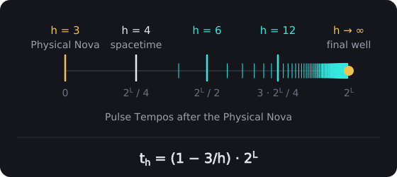
Data Harmonics. Counted from the Physical Nova, Harmonic h arrives at t_h = (1 − 3/h) · 2ᴸ Tempos: spacetime (h = 4) at a quarter of the life, h = 6 at a half, h = 12 at three quarters. The gaps, 3 · 2ᴸ / (h(h − 1)) Tempos, shrink toward zero, and the later harmonics crowd into the final well.
Layer Count Law G
h⥣(L) = 3 · 2^L [∅]
Dimensional analysis:
Where (from the book): h⥣ [∅], L [∅], 2^L [∅]
[∅]([∅]) = [∅]
[∅] × [∅] = [∅]
[∅] = [∅] ✓ Valid PulseCore Verified ✓
A universe of level L reaches Harmonic 3·2^L before its final well; the last harmonics arrive together as its life closes
Where:
- h⥣ [∅] — the highest harmonic a universe reaches in its life, the Null Nova counted as Harmonic 1 and the Data Nova as Harmonic 2
- L [∅] — the universe's level in the UniSphere
- 2^L [∅] — the universe's life in Pulse Tempos, here counted
➢ Harmonic h falls within the life while it arrives before the final well, at the latest in the life's last Tempo: (1 − 3/h)·2^L ≤ 2^L − 1, so h ≤ 3·2^L. The count of distinct arrivals is smaller, about twice √(3·2^L), because the later harmonics come within one Tempo of each other and arrive together.
The law reads directly. Level 0, the Zinf, reaches h⥣(0) = 3 · 2⁰ = 3: its Null Nova and its Data Nova come at the second and third steps of its Pulsecore's count and take no universe time, and Harmonic 3, the physical, arrives as its one-Tempo life begins (t₃ = (1 − 3/3) · 2⁰ = 0), which is also its last Tempo, so it holds three layers, the toroidal form, its data and the physical, and no spacetime. Level 1, with h⥣(1) = 6, is the first to reach spacetime, Harmonic 4, at t₄ = (1 − 3/4) · 2 = ½ Tempo, and so the first to complete the fourfold scaffold; Harmonics 5 and 6 follow at 0.8 and 1 Tempo, the last in the final Tempo of its two-Tempo life. The First Fork (Part 3.10), the first universe able to hold two wells and to spin, comes at level 3. Our Universe at level 202 reaches Harmonic 3·2^202: four dimensional layers and the rest harmonic, the last arriving together as its life closes, at its final well.
The layers after saturation are inner dimensions. They open no new direction of space or time, but they are part of what a universe consists of: the harmonic modes listed above. A deeper universe holds more of them. The law also bounds the binding rule left open earlier in this Part: whatever sets D⥣, it cannot exceed 3·2^L. A Nova is a discharge, not a collapse: Novas open layers, while wells form by collapse (Null Well Collapse, Part 3.9).
3.6 Testable Predictions
- Toroidal Boundary Imprint in CMB: If the Null Nova formed toroidal containment, Cosmic Microwave Background should preserve subtle anisotropies consistent with closed-loop topology rather than isotropic singular expansion, detectable through CMB map analysis (Planck Collaboration, 2020).
- Quantization of Dimensional Transitions: Dimensional growth occurs in discrete "nova jumps," not continuously. This would leave measurable signatures of abrupt phase transitions in the early Universe, observable through discontinuities in early cosmic structure distribution.
- Resonant Gravity as Harmonic Mode: Gravity is not force "on top" of spacetime but a resonance field arising from toroidal harmonics. Gravitational interactions should exhibit harmonic frequency signatures at extreme scales, detectable through resonance-like modulations in gravitational wave spectra (Abbott et al., 2016)¹.
- Entanglement as Phase-Locked Toroidal Resonance: Quantum entanglement results from phase-locking across toroidal loops. Entangled systems should exhibit coherence patterns depending on toroidal geometry, not spatial separation.
- Dimensional Saturation at D=4: At our depth, no physical phenomena should require more than four coherent dimensions (three spatial + one temporal) to model accurately. Attempts extending beyond four should reduce back into harmonic reinforcement rather than independent dimensions, the etheric harmonics of Part 4.8. The count is measured, not only predicted: our universe's ratio of dark matter to ordinary matter gives D = 3.85 (+0.23 / −0.20) (Part 3.13).
- A Preferred Axis from the Throat: If our Universe is a torus whose data circulates up through its throat, the Null Vacuum left by the Data Nova, and back round the outside (the Data Loop), then everything we see streams out of one origin along one axis: the Big Bang as it appears to us looking back toward our Data Nova. The sky should then carry a preferred axis at the largest scales instead of perfect isotropy. The lowest multipoles of the Cosmic Microwave Background, the quadrupole and the octopole, should align with each other and with the axis of the hemispherical power asymmetry, the alignment reported as the "axis of evil" (Land & Magueijo, 2005) and seen at modest significance in Planck's isotropy tests (Planck Collaboration, 2020). The prediction fails if these large-scale anomalies fade to chance in future full-sky data, or if their axes turn out to be unrelated to one another.
Toroidal Genesis proposes that dimensions aren't given — they're created through computational overflow events. The Universe literally computes its own dimensional structure through Data Nova Escalation, building reality's architecture through stepwise dimensional layering. We inhabit not a mysterious four-dimensional spacetime but a computationally constructed geometric substrate; why that construction presents 3 + 1 dimensions at our depth remains an open question of the theory.