Chapter 6 · Section 5
Density and the Relative Planck Constant
The physical picture of density-dependent constants is set out in Part 2.5; here we give its formal structure.
Density-Dependent Constant Framework & Planck Time Scaling
Planck's natural units (Planck, 1899) established conventional Planck time, but BPT holds that this is incomplete. By examining the Standard Planck Time, Density-Modified Planck Time, Scaling Function, Complete Density-Time Relation, and Modified Pulse Rhythm we can understand how density-dependent constant framework operates through local temporal quantization depending on collapse conditions that reframe our understanding of time itself, while Planck time scaling shows how higher collapse density yields shorter pulse time with faster temporal resolution and lower collapse density yields longer pulse time with slower temporal resolution.
This demonstrates modification cascades into structural emergence rates that address fine-tuning problems by proposing that constants emerge from computational heritage rather than arbitrary universal principles through density-dependent temporal scaling mechanisms.
Standard Planck Time
t_P = sqrt(ℏG/c⁵) ≈ 5.39 × 10⁻⁴⁴ seconds [𝕋]
Where:
- t_P [𝕋] - standard Planck time
- ℏ [𝕄·𝕃²·𝕋⁻¹] - reduced Planck constant
- G [𝕄⁻¹·𝕃³·𝕋⁻²] - gravitational constant
- c [𝕃·𝕋⁻¹] - speed of light
- sqrt [∅] - square root function
➢ Planck's natural units (Planck, 1899) established conventional Planck time, but BPT holds that this is incomplete and adds density-dependent modifications.
In BPT, local Planck time becomes density-dependent through Null Well collapse characteristics.
Density-Modified Planck Time
①⥂⧗'⌂ = ①⥂⧗⌂ · fρ(ρ⦰) [𝕋]
Where:
- ①⥂⧗'⌂ [𝕋] - density-modified Pulse Tempo
- ①⥂⧗⌂ [𝕋] - Local Pulse Tempo (standard Planck time)
- fρ [∅] - density scaling function
- ρ⦰ [𝕄·𝕃⁻³] - density at Null Well formation
Dimensional analysis:
Where (from the book): fρ [∅], ρ⦰ [𝕄·𝕃⁻³]
[𝕋]
[𝕋] × [∅]([𝕄·𝕃⁻³]) = [𝕋] × [∅] = [𝕋]
[𝕋] = [𝕋] ✓ Valid PulseCore Verified ✓
➢ Local temporal quantization depends on collapse conditions, reframing our understanding of time itself where Planck time becomes density-dependent through Null Well collapse characteristics.
Scaling Function
fρ(ρ) = (ρ_P/ρ⦰)^(1/2) [∅]
Where:
- fρ(ρ) [∅] - density scaling function
- ρ_P [𝕄·𝕃⁻³] - Planck density
- ρ⦰ [𝕄·𝕃⁻³] - collapse density
Dimensional analysis:
Where (from the book): fρ(ρ) [∅], ρ_P [𝕄·𝕃⁻³], ρ⦰ [𝕄·𝕃⁻³]
[∅]
([𝕄·𝕃⁻³] ÷ [𝕄·𝕃⁻³])^([∅] ÷ [∅]) = ([𝕄·𝕃⁻³] ÷ [𝕄·𝕃⁻³])^([∅]) = [∅]^([∅]) = [∅]
[∅] = [∅] ✓ Valid PulseCore Verified ✓
➢ The relationship yields the key result where density ratio determines temporal scaling through square root dependence on collapse conditions.
Complete Density-Time Relation
①⥂⧗'⌂ = sqrt(ℏG·ρ_P/(𝒞→⁵·ρ⦰)) [𝕋]
Where:
- ①⥂⧗'⌂ [𝕋] - density-modified Pulse Tempo
- ℏ [𝕄·𝕃²·𝕋⁻¹] - reduced Planck constant
- G [𝕄⁻¹·𝕃³·𝕋⁻²] - gravitational constant
- ρ_P [𝕄·𝕃⁻³] - Planck density
- 𝒞→ [𝕃·𝕋⁻¹] - speed of light
- ρ⦰ [𝕄·𝕃⁻³] - collapse density
➢ Higher collapse density → shorter Pulse Tempo → faster child; lower collapse density → longer Pulse Tempo → slower child. Slower is the rule. A single collapse does not compress its core past the parent's Planck density, so ρ⦰ ≤ ρ_P and the child pulses more slowly than its parent. A core passes that density only with help: the merger compression of Part 6.8, or the merger-built core of a supermassive well. A supermassive well is the least dense on average, since mean density falls as 1/M², so it is its core, not its size, that can give a faster child. No core passes the Zinf limit, so every Tempo stays at or above ℨ and the Zinf universe remains the fastest.
Zinf Tempo Floor
①⥂⧗'⌂ ≥ ℨ
Dimensional analysis:
[𝕋] ≥ [ℨ] ✓ Valid PulseCore Verified ✓
➢ The fast branch is bounded: a child can step back up the ladder toward the Zinf universe but never past it.
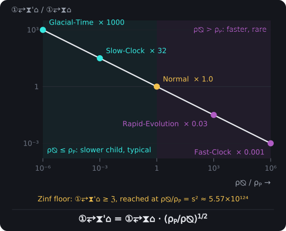
Density and the Child's Pulse Tempo. A child universe's Pulse Tempo scales as ①⥂⧗'⌂ = ①⥂⧗⌂ · (ρ_P/ρ⦰)^½. A single collapse stays at or below the Planck density and gives a slower child; only merger or supermassive cores pass it and give a faster one, never faster than the Zinf ℨ, which would need ρ⦰/ρ_P = s² ≈ 5.57 × 10¹²⁴.
Since ①⥂⧖⌂ = ①⥂⧗⌂/2 from established frameworks, density modification directly affects Pulse Rhythm.
Modified Pulse Rhythm
①⥂⧖'⌂ = ①⥂⧗'⌂/2 = ①⥂⧖⌂ · (ρ_P/ρ⦰)^(1/2) [𝕋]
Where:
- ①⥂⧖'⌂ [𝕋] - modified Pulse Rhythm
- ①⥂⧗'⌂ [𝕋] - density-modified Pulse Tempo
- ①⥂⧖⌂ [𝕋] - baseline Pulse Rhythm
- ρ_P [𝕄·𝕃⁻³] - Planck density
- ρ⦰ [𝕄·𝕃⁻³] - collapse density
Dimensional analysis:
Where (from the book): ρ_P [𝕄·𝕃⁻³], ρ⦰ [𝕄·𝕃⁻³]
[𝕋]
[𝕋] ÷ [∅] = [𝕋]
[𝕋] × ([𝕄·𝕃⁻³] ÷ [𝕄·𝕃⁻³])^([∅] ÷ [∅]) = [𝕋] × ([𝕄·𝕃⁻³] ÷ [𝕄·𝕃⁻³])^([∅]) = [𝕋] × [∅]^([∅]) = [𝕋] × [∅] = [𝕋]
[𝕋] = [𝕋] = [𝕋] ✓ Valid PulseCore Verified ✓
➢ Modification cascades into structural emergence rates, addressing the fine-tuning problem by proposing that constants emerge from computational heritage where Pulse Rhythm scaling affects temporal resolution.
The Standard Planck Time, Density-Modified Planck Time, Scaling Function, Complete Density-Time Relation, and Modified Pulse Rhythm establish how density-dependent constant framework functions through local temporal quantization depending on collapse conditions that reframe our understanding of time itself, demonstrating Planck time becomes density-dependent through Null Well collapse characteristics where density scaling function determines temporal modification through square root dependence, yielding complete density-time relation where higher collapse density produces shorter pulse time with faster temporal resolution while lower collapse density produces longer pulse time with slower temporal resolution.
This enables Pulse Rhythm modification that cascades into structural emergence rates and addresses fine-tuning problems by proposing that constants emerge from computational heritage rather than arbitrary universal principles through density-dependent temporal scaling mechanisms that connect collapse conditions to fundamental constant modification.
Fundamental Constant Modulation Framework
Since Planck units are combinatorial functions of ℏ, G, c, variation in ①⥂⧗'⌂ necessitates corresponding modifications. By examining the Modified Fundamental Constants, Consistency Constraint, Scaling Function Constraint, Scaling Function Specifications, and Dimensional Consistency Requirement we can understand how fundamental constant modulation framework operates through density-dependent scaling functions that modify Planck constant, gravitational constant, and speed of light while maintaining consistency constraint for modified Planck time calculation.
This demonstrates scaling function constraint ensures mathematical consistency and dimensional consistency requirement provides unified parameter modulation framework that connects scaling relationships from previous parts and ensures coherent constant modification across density-dependent parameter inheritance.
Modified Fundamental Constants:
Planck Constant
ℏ' = ℏ · g₁(ρ⦰) [𝕄·𝕃²·𝕋⁻¹]
Dimensional analysis:
[𝕄·𝕃²·𝕋⁻¹]
[𝕄·𝕃²·𝕋⁻¹] × [∅]([𝕄·𝕃⁻³]) = [𝕄·𝕃²·𝕋⁻¹] × [∅] = [𝕄·𝕃²·𝕋⁻¹]
[𝕄·𝕃²·𝕋⁻¹] = [𝕄·𝕃²·𝕋⁻¹] ✓ Valid PulseCore Verified ✓
Gravitational Constant
G' = G · g₂(ρ⦰) [𝕄⁻¹·𝕃³·𝕋⁻²]
Dimensional analysis:
[𝕄⁻¹·𝕃³·𝕋⁻²]
[𝕄⁻¹·𝕃³·𝕋⁻²] × [∅]([𝕄·𝕃⁻³]) = [𝕄⁻¹·𝕃³·𝕋⁻²] × [∅] = [𝕄⁻¹·𝕃³·𝕋⁻²]
[𝕄⁻¹·𝕃³·𝕋⁻²] = [𝕄⁻¹·𝕃³·𝕋⁻²] ✓ Valid PulseCore Verified ✓
Speed of Light
𝒞→' = 𝒞→ · g₃(ρ⦰) [𝕃·𝕋⁻¹]
Where:
- ℏ' [𝕄·𝕃²·𝕋⁻¹] - modified Planck constant
- ℏ [𝕄·𝕃²·𝕋⁻¹] - original Planck constant
- g₁(ρ⦰) [∅] - Planck constant scaling function
- G' [𝕄⁻¹·𝕃³·𝕋⁻²] - modified gravitational constant
- G [𝕄⁻¹·𝕃³·𝕋⁻²] - original gravitational constant
- g₂(ρ⦰) [∅] - gravitational constant scaling function
- 𝒞→' [𝕃·𝕋⁻¹] - modified speed of light
- 𝒞→ [𝕃·𝕋⁻¹] - original speed of light
- g₃(ρ⦰) [∅] - light speed scaling function
- ρ⦰ [𝕄·𝕃⁻³] - collapse density
Dimensional analysis:
Where (from the book): ℏ [𝕄·𝕃²·𝕋⁻¹], g₁(ρ⦰) [∅], G' [𝕄⁻¹·𝕃³·𝕋⁻²], G [𝕄⁻¹·𝕃³·𝕋⁻²], g₂(ρ⦰) [∅], g₃(ρ⦰) [∅], ρ⦰ [𝕄·𝕃⁻³]
[𝕃·𝕋⁻¹]
[𝕃·𝕋⁻¹] × [∅] = [𝕃·𝕋⁻¹]
[𝕃·𝕋⁻¹] = [𝕃·𝕋⁻¹] ✓ Valid PulseCore Verified ✓
➢ Since Planck units are combinatorial functions of ℏ, G, c, variation in ①⥂⧗'⌂ necessitates corresponding modifications through density-dependent scaling functions. In the terms of Part 6.2, g₁ = δ = (①⥂⧗′⌂/①⥂⧗⌂)², g₃ = β and g₂ = γ = g₃⁵ (Constants of a Child Universe, Chapter 1).
➢ Read by the Data Light Speed Relation (Chapter 1), this is light speed compared between universes in one frame. Each universe measures its own as one Pulse Length per Tempo, 𝒞→ in its own units. On the typical ladder the Length and the Tempo grow together and the scaling is 1; it differs from 1 only off the ladder, where a child's Tempo comes from its Null Well's mass and its Length from its parent's singularity. In the UniSphere's own frame, pixels crossed per Zinf cycle, every universe's light moves at 1/s of its data, so a child's light, set beside its parent's, moves at s/s′ of it.
Consistency Constraint
①⥂⧗'⌂ = sqrt(ℏ'G'/𝒞→'⁵) [𝕋]
Where:
- ①⥂⧗'⌂ [𝕋] - modified Pulse Tempo
- ℏ' [𝕄·𝕃²·𝕋⁻¹] - modified Planck constant
- G' [𝕄⁻¹·𝕃³·𝕋⁻²] - modified gravitational constant
- 𝒞→' [𝕃·𝕋⁻¹] - modified speed of light
➢ Consistency constraint ensures modified Planck time calculation remains valid with modified fundamental constants through combinatorial relationships.
Scaling Function Constraint
g₁(ρ) · g₂(ρ) = g₃(ρ)⁵ · (ρ_P/ρ⦰) [∅]
Where:
- g₁(ρ) [∅] - Planck constant scaling function
- g₂(ρ) [∅] - gravitational constant scaling function
- g₃(ρ) [∅] - light speed scaling function
- ρ [𝕄·𝕃⁻³] - density
- ρ_P [𝕄·𝕃⁻³] - Planck density
- ρ⦰ [𝕄·𝕃⁻³] - Null Well collapse density that sets the child's Tempo
Dimensional analysis:
Where (from the book): g₁(ρ) [∅], g₂(ρ) [∅], g₃(ρ) [∅], ρ [𝕄·𝕃⁻³]
[∅] × [∅] = [∅]
[∅]
[∅] = [∅] ✓ Valid PulseCore Verified ✓
➢ Scaling function constraint ensures mathematical consistency between density-dependent modifications of fundamental constants through constraint relationship.
Scaling Function Specifications
g₁(ρ) = (ρ_P/ρ)^α [∅]
Dimensional analysis:
[∅]([𝕄·𝕃⁻³]) = [∅]
([𝕄·𝕃⁻³] ÷ [𝕄·𝕃⁻³])^([∅]) = [∅]^([∅]) = [∅]
[∅] = [∅] ✓ Valid PulseCore Verified ✓
g₂(ρ) = (ρ_P/ρ)^β [∅]
Dimensional analysis:
[∅]([𝕄·𝕃⁻³]) = [∅]
([𝕄·𝕃⁻³] ÷ [𝕄·𝕃⁻³])^([∅]) = [∅]^([∅]) = [∅]
[∅] = [∅] ✓ Valid PulseCore Verified ✓
g₃(ρ) = (ρ_P/ρ)^γ [∅]
Where:
- ρ_P [𝕄·𝕃⁻³] - Planck density
- α, β, γ [∅] - density scaling exponents
Dimensional analysis:
Where (from the book): ρ_P [𝕄·𝕃⁻³], α, [∅]
[∅]([𝕄·𝕃⁻³]) = [∅]
([𝕄·𝕃⁻³] ÷ [𝕄·𝕃⁻³])^([∅]) = [∅]^([∅]) = [∅]
[∅] = [∅] ✓ Valid PulseCore Verified ✓
➢ Scaling function specifications show density ratio dependence with exponents determining parameter inheritance through power law relationships.
Dimensional Consistency Requirement
α + β − 5γ = 1 [∅]
Where:
- α [∅] - Planck constant scaling exponent
- β [∅] - gravitational constant scaling exponent
- γ [∅] - light speed scaling exponent
Dimensional analysis:
Where (from the book): α [∅], β [∅], γ [∅]
[∅] + [∅] = [∅]
[∅] × [∅] = [∅]
[∅] = [∅] ✓ Valid PulseCore Verified ✓
➢ Functions correspond to scaling relationships from Parts 6.3-6.4, providing a unified parameter modulation framework where dimensional consistency requirement ensures mathematical coherence across constant modifications.
The Modified Fundamental Constants, Consistency Constraint, Scaling Function Constraint, Scaling Function Specifications, and Dimensional Consistency Requirement establish how fundamental constant modulation framework functions through density-dependent scaling functions that modify fundamental constants while maintaining mathematical consistency, demonstrating variation in modified Planck time necessitates corresponding modifications where consistency constraint ensures valid Planck time calculation and scaling function constraint maintains mathematical coherence between density-dependent modifications.
This provides a unified parameter modulation framework through dimensional consistency requirement that connects scaling relationships from previous parts and ensures coherent constant modification across density-dependent parameter inheritance through power law relationships and exponent constraints that govern fundamental constant evolution in emergent universes.
Domain-Specific Physics and Universe Classification
By examining the Quantum Scale Modifications, Gravitational Scale Modifications, and Universe Classification framework we can understand how modified constants create unique physical environments within each Universe domain where density regimes determine temporal scaling and physical law modifications, while classification system categorizes universes from Ultra-High density Fast-Clock types to Ultra-Low density Glacial-Time types based on Planck time and Pulse Rhythm ratios.
Physical Law Modifications
Within each Universe domain, modified constants create unique physical environments.
Quantum Scale Modifications:
Compton Wavelength
λ'_C = ℏ'/(m'𝒞→') = λ_C · (ℏ'/ℏ) · (𝒞→/𝒞→') [𝕃]
Bohr Radius
a'₀ = ℏ'²/(m'e²) = a₀ · (ℏ'/ℏ)² [𝕃]
Fine Structure Constant
α' = e²/(4πε₀ℏ'𝒞→') = α · (ℏ/ℏ') · (𝒞→/𝒞→') [∅]
Where:
- λ'_C [𝕃] - modified Compton wavelength
- ℏ' [𝕄·𝕃²·𝕋⁻¹] - modified Planck constant
- m' [𝕄] - modified particle mass
- 𝒞→' [𝕃·𝕋⁻¹] - modified speed of light
- λ_C [𝕃] - original Compton wavelength
- ℏ [𝕄·𝕃²·𝕋⁻¹] - original Planck constant
- 𝒞→ [𝕃·𝕋⁻¹] - original speed of light
- a'₀ [𝕃] - modified Bohr radius
- e [∅] - elementary charge
- a₀ [𝕃] - original Bohr radius
- α' [∅] - modified fine structure constant
- ε₀ [M⁻¹L⁻³T⁴A²] - permittivity of free space
- α [∅] - original fine structure constant
Gravitational Scale Modifications:
Schwarzschild Radius
r'_s = 2G'M/𝒞→'² = r_s · (G'/G) · (𝒞→/𝒞→')² [𝕃]
Gravitational Coupling
g'⇅ = G'm²/(ℏ'𝒞→') = g⇅ · (G'/G) · (ℏ/ℏ') · (𝒞→/𝒞→') [∅]
Where:
- r'_s [𝕃] - modified Schwarzschild radius
- G' [𝕄⁻¹·𝕃³·𝕋⁻²] - modified gravitational constant
- M [𝕄] - mass
- 𝒞→' [𝕃·𝕋⁻¹] - modified speed of light
- r_s [𝕃] - original Schwarzschild radius
- G [𝕄⁻¹·𝕃³·𝕋⁻²] - original gravitational constant
- 𝒞→ [𝕃·𝕋⁻¹] - original speed of light
- g'⇅ [∅] - modified gravitational coupling
- m [𝕄] - particle mass
- ℏ [𝕄·𝕃²·𝕋⁻¹] - original Planck constant
- g⇅ [∅] - original gravitational coupling
- ℏ' [𝕄·𝕃²·𝕋⁻¹] - modified Planck constant
➢ Gravitational scale modifications show how black hole formation and gravitational interactions change through modified gravitational constant, Planck constant, and speed of light affecting Schwarzschild radius and gravitational coupling strength in emergent universes.
Universe Classification by Density Regimes
Density Range | ρ/ρ_P | ①⥂⧗'⌂/①⥂⧗⌂ | ①⥂⧖'⌂/①⥂⧖⌂ | Universe Type |
|---|---|---|---|---|
Ultra-High | 10⁶ | 10⁻³ | 10⁻³ | Fast-Clock (rare: merger or supermassive cores) |
High | 10³ | 0.03 | 0.03 | Rapid-Evolution (rare: merger cores) |
Standard | 1 | 1.0 | 1.0 | Normal (the parent's own Tempo) |
Low | 10⁻³ | 32 | 32 | Slow-Clock (typical) |
Ultra-Low | 10⁻⁶ | 10³ | 10³ | Glacial-Time (typical) |
Where:
- ρ/ρ_P [∅] - density ratio to Planck density
- ①⥂⧗'⌂/①⥂⧗⌂ [∅] - modified to original Pulse Tempo ratio
- ①⥂⧖'⌂/①⥂⧖⌂ [∅] - modified to original Pulse Rhythm ratio
Dimensional analysis: All ratios are [∅]/[∅] = [∅] ✓ Universe classification framework uses dimensionless ratios for categorization.
➢ Universe classification by density regimes demonstrates systematic categorization from Ultra-High density Fast-Clock universes with rapid temporal evolution to Ultra-Low density Glacial-Time universes with extremely slow temporal progression through Pulse Rhythm scaling.
The Quantum Scale Modifications, Gravitational Scale Modifications, and Universe Classification Framework establish how domain-specific physics functions through modified constants creating unique physical environments where quantum and gravitational phenomena scale differently in emergent universes, demonstrating systematic modifications to Compton wavelength, Bohr radius, fine structure constant, Schwarzschild radius, and gravitational coupling through density-dependent constant ratios that enable universe classification by density regimes ranging from Fast-Clock to Glacial-Time types.
This provides comprehensive framework for understanding how fundamental physics changes across different universe domains through density-dependent parameter inheritance where quantum scale modifications affect atomic and particle physics while gravitational scale modifications alter black hole formation and gravitational interactions, enabling systematic classification based on density ratios that determine temporal evolution rates and physical law modifications through modified Planck time and Pulse Rhythm scaling relationships.
Intra-Domain Constancy versus Inter-Domain Variation
Constants appear fixed within single domains due to homogeneous recursive inheritance, but jump discontinuously at Null Well interfaces.
Within Single Domains:
- Causal synchronization maintains uniform Pulse rates
- Local physics follows standard quantum/relativistic laws
Across Domain Boundaries:
- Constants jump discontinuously at Null Well interfaces
- Cross-domain communication requires Constant Conversion Protocols
Relativistic Consistency and Multiverse Structure
By examining the Standard General Relativity and BPT Computational Analog we can see how BPT seeks a Pulse-rate account of gravitational time dilation that would provide a computational foundation for relativistic effects, connecting established temporal frameworks with density-dependent time scaling relationships.
Gravitational Time Dilation Foundation
BPT seeks a Pulse-rate account of gravitational time dilation. The ratio sqrt(ρ_P/ρ⌂) below is a child universe's Tempo across a Null Well, not dt'/dt at a radius r inside our universe; a weak-field map ρ(r) ↔ 1 − r_s/r is open.
Standard General Relativity
dt'/dt = sqrt(1 - 2GM/(rc²)) [∅]
Where:
- dt' [𝕋] - proper time interval
- dt [𝕋] - coordinate time interval
- G [𝕄⁻¹·𝕃³·𝕋⁻²] - gravitational constant
- M [𝕄] - gravitational mass
- r [𝕃] - radial distance
- c [𝕃·𝕋⁻¹] - speed of light
- sqrt [∅] - square root function
➢ Standard general relativity describes gravitational time dilation through metric tensor effects where proper time relates to coordinate time through gravitational potential.
BPT Computational Analog
dt'/dt = ①⥂⧗'⌂/①⥂⧗⌂ = sqrt(ρ_P/ρ⌂) [∅]
Where:
- dt'/dt [∅] - time dilation ratio
- ①⥂⧗'⌂ [𝕋] - modified Pulse Tempo
- ①⥂⧗⌂ [𝕋] - Local Pulse Tempo (standard Planck time)
- ρ_P [𝕄·𝕃⁻³] - Planck density
- ρ⌂ [𝕄·𝕃⁻³] - local density
Dimensional analysis:
Where (from the book): dt'/dt [∅], ρ_P [𝕄·𝕃⁻³], ρ⌂ [𝕄·𝕃⁻³]
[∅]
[𝕋] ÷ [𝕋] = [∅]
sqrt([𝕄·𝕃⁻³] ÷ [𝕄·𝕃⁻³]) = sqrt([∅]) = [∅]
[∅] = [∅] = [∅] ✓ Valid PulseCore Verified ✓
➢ BPT provides computational foundation for relativistic effects through Pulse (G) rate modulation, connecting to established temporal frameworks where density-dependent Planck time scaling seeks to account for gravitational time dilation.
The Standard General Relativity and BPT Computational Analog establish how BPT seeks a Pulse-rate account of gravitational time dilation as a computational foundation for relativistic effects: standard general relativity describes time dilation through gravitational potential, while the BPT computational analog proposes the same effects through density-dependent Planck time scaling where local energy density determines temporal modulation, connecting established temporal frameworks with computational substrate architecture that enables relativistic consistency through density ratio calculations equivalent to metric tensor effects in general relativity.
6.5 Testable Predictions
The predictions this part shares with Chapter 2 are listed in Part 2.5.
If confirmed, these predictions would indicate that:
- Multiple Universes exist with systematically varying physics