Chapter 7 · Section 1
Harmonic Complexity and the Recursive Spectrum
How do harmonics emerge when the underlying medium is not a continuous vibrating string, but a discrete computational substrate? Classical wave theory describes the harmonic series as integer multiples of a fundamental frequency, where for a fundamental tone f_0, the nth harmonic follows f_n = n × f_0, creating linear additive overtone structures characteristic of vibrating strings, air columns, and bounded periodic media (Fletcher & Rossing, 1998)¹.
Binary Pulse Theory fundamentally reconceptualizes this framework by introducing Recursive Complexity Growth that generates Nonlinear Harmonic Spectra reflecting the underlying computational architecture of the binary substrate established in Parts 5.1-5.5. Rather than simple linear progression, BPT harmonics emerge from Prime Pulse Bifurcation mechanisms operating through Recursive State Evolution, where each generation inherits and amplifies the computational load of previous cycles, extending principles found in acoustic systems (Kinsler et al., 2000)².
Mathematical Foundation of Recursive Harmonic Architecture
By examining the Computational Load Accumulation and Simplified Load Function relationships, we can understand how recursive processing requirements grow quadratically with recursion depth, revealing the mathematical foundation for harmonic complexity scaling that drives temporal drag effects through systematic accumulation of structural complexity and information conservation mechanisms in computational substrate evolution.
Harmonic Frequency Scaling demonstrates how this quadratic growth manifests in frequency domain evolution, with harmonic frequencies scaling as (n+1)² rather than following linear relationships, revealing the computational substrate architecture's fundamental influence on frequency evolution through recursive complexity accumulation that connects computational load growth directly to pulse density evolution and temporal drag phenomena in Binary Pulse Theory. Unlike classical harmonic systems where overtones follow linear spacing, BPT establishes complexity scaling based on the following.
Computational Load Accumulation G
L(n) = L_0 + sum(k=1 to n) k = L_0 + n(n+1)/2 [∅]
Where:
- L(n) [∅] - cumulative computational load
- L_0 [∅] - initial processing overhead
- sum(k=1 to n) - summation operator from k=1 to n
- k [∅] - processing cost at step k
- n [∅] - recursion depth
- [∅] - quantities without physical units, pure numerical ratios or mathematical constants
➢ Each recursive step must process all previous states, creating quadratic growth in computational requirements that drives Harmonic Complexity Scaling through systematic accumulation of processing overhead across recursive substrate evolution. This works for systems where the initial load is negligible (L_0 << n(n+1)/2 for n >> 1):
Simplified Load Function
L(n) ≈ n(n+1)/2 [∅]
Dimensional analysis:
[∅] ≈ [∅]([∅] + [∅]) ÷ [∅] = [∅] ≈ [∅]([∅]) ÷ [∅] = [∅] ≈ [∅] ÷ [∅] = [∅] ≈ [∅] ✓ Valid PulseCore Verified ✓
Pulse Density Function
P(n) = (n + 1)² [∅]
Where:
- L(n) [∅] - simplified cumulative computational load
- P(n) [∅] - pulse density function
- n [∅] - recursion depth index
- [∅] - quantities without physical units, pure numerical ratios or mathematical constants
Dimensional analysis:
Where (from the book): n [∅], [∅] [∅]
[∅]
([∅] + [∅])² = [∅]² = [∅]
[∅] = [∅] ✓ Valid PulseCore Verified ✓
➢ Quadratic scaling reflects recursive accumulation of structural complexity per Pulse iteration through Information Conservation mechanisms; P(n) = (n+1)² is the harmonic model's postulate, and L(n) = n(n+1)/2 ≈ P(n)/2 motivates it.
Harmonic Frequency Scaling
H_n = ν_0 × P(n) = ν_0 × (n + 1)² [𝕋⁻¹]
Where:
- H_n [𝕋⁻¹] - nth harmonic frequency
- ν_0 [𝕋⁻¹] - fundamental Pulse frequency, equal to 1/①⥂⧗⌂ (the Initial Pulse Frequency of Part 7.4, ≈ 1.855 × 10⁴³ Hz)
- P(n) [∅] - quadratic complexity function
- n [∅] - harmonic index
- ①⥂⧗⌂ [𝕋] - Local Pulse Tempo (Planck time)
- [∅] - quantities without physical units, pure numerical ratios or mathematical constants
Dimensional analysis:
Where (from the book): n [∅], [∅] [∅]
[𝕋⁻¹]
[𝕋⁻¹] × [∅] = [𝕋⁻¹]
[𝕋⁻¹] × ([∅] + [∅])² = [𝕋⁻¹] × [∅]² = [𝕋⁻¹] × [∅] = [𝕋⁻¹]
[𝕋⁻¹] = [𝕋⁻¹] = [𝕋⁻¹] ✓ Valid PulseCore Verified ✓
➢ Harmonic frequencies scale quadratically rather than linearly, reflecting computational substrate architecture where recursive complexity accumulation drives frequency evolution through Information Conservation mechanisms in the underlying Binary Pulse framework. These harmonics, indexed by n with H_n = ν_0 × (n + 1)², are distinct from the Data Harmonics of Part 3.6, whose index counts octaves (T_n = 2^(n−1) × T₁); the two share a name, not an n.
The Computational Load Accumulation framework demonstrates how Binary Pulse Theory explains temporal drag through quadratic scaling of computational requirements, with each recursive step processing all previous states while connecting computational complexity to pulse evolution through fundamental information conservation mechanisms in the substrate architecture.
Harmonic Frequency Scaling reveals how this quadratic growth creates systematic deviations from linear harmonic relationships, with frequencies scaling as (n+1)² rather than linearly, fundamentally connecting frequency evolution to computational load growth through recursive complexity accumulation that manifests as harmonic complexity scaling and temporal deceleration effects.
Frequency Structure and Spectral Characteristics
By studying the Recursive Frequency Spacing and Spectral Density Function, we can understand how frequency intervals between consecutive harmonics increase linearly with recursion depth rather than remaining constant, creating discrete spectral lines positioned according to quadratic frequency scaling with energy weighting that produce characteristic signatures distinguishing Binary Pulse Theory harmonic structures from classical systems.
The Harmonic Energy Distribution reveals how energy allocation across harmonics must decay faster than quadratic growth to ensure physical realizability, with convergence requiring γ > 3 for finite total energy, demonstrating the fundamental constraints that govern energy distribution in recursive harmonic systems and ensure mathematical consistency in computational substrate architectures. Recursive Frequency Spacing deviates from uniform intervals through computational complexity scaling.
Recursive Frequency Spacing G
Δf_n = H_(n+1) - H_n = ν_0 × [(n + 2)² - (n + 1)²] = ν_0 × (2n + 3) [𝕋⁻¹]
Where:
- Δf_n [𝕋⁻¹] - frequency spacing between consecutive harmonics
- H_(n+1) [𝕋⁻¹] - (n+1)th harmonic frequency
- H_n [𝕋⁻¹] - nth harmonic frequency
- ν_0 [𝕋⁻¹] - fundamental Pulse frequency
- n [∅] - harmonic index
- [∅] - quantities without physical units, pure numerical ratios or mathematical constants
Dimensional analysis:
Where (from the book): n [∅], [∅] [∅]
Read dimensionally: Δf_n = H_(n+1) - H_n = ν_0 × ((n + 2)² - (n + 1)²) = ν_0 × (2n + 3)
[𝕋⁻¹]
[𝕋⁻¹] - [𝕋⁻¹] = [𝕋⁻¹]
[𝕋⁻¹] × (([∅] + [∅])² - ([∅] + [∅])²) = [𝕋⁻¹] × ([∅]² - ([∅] + [∅])²) = [𝕋⁻¹] × ([∅] - ([∅] + [∅])²) = [𝕋⁻¹] × ([∅] - [∅]²) = [𝕋⁻¹] × ([∅] - [∅]) = [𝕋⁻¹] × [∅] = [𝕋⁻¹]
[𝕋⁻¹] × ([∅] × [∅] + [∅]) = [𝕋⁻¹] × ([∅] + [∅]) = [𝕋⁻¹] × [∅] = [𝕋⁻¹]
[𝕋⁻¹] = [𝕋⁻¹] = [𝕋⁻¹] = [𝕋⁻¹] ✓ Valid PulseCore Verified ✓
➢ Frequency intervals increase linearly with recursion depth, unlike constant intervals in classical harmonics, demonstrating how computational substrate architecture creates systematic spacing variations that reflect underlying recursive complexity accumulation.
Spectral Density Function
σ(f) = sum_n δ(f - H_n) E_n [J·s]
Where:
- σ(f) [J·s] - Spectral Density Function
- sum_n - summation operator over all harmonic indices n
- δ [𝕋] - Dirac delta function
- f [𝕋⁻¹] - frequency variable
- H_n [𝕋⁻¹] - nth harmonic frequency
- E_n [J] - energy of nth harmonic
- n [∅] - harmonic index
- [∅] - quantities without physical units, pure numerical ratios or mathematical constants
➢ Discrete spectral lines positioned according to quadratic frequency scaling with energy weighting, creating characteristic spectral signatures that encode recursive computational complexity and distinguish BPT harmonic structures from classical constant-interval systems.
Harmonic Energy Distribution
E_n = E_0 × (n + 1)^(2-γ) [J]
Where:
- E_n [J] - energy of nth harmonic
- E_0 [J] - fundamental energy scale
- n [∅] - harmonic index
- γ [∅] - Convergence Parameter
- ^(2-γ) [∅] - power law exponent
- [∅] - quantities without physical units, pure numerical ratios or mathematical constants
Dimensional analysis:
Where (from the book): E_n [J], E_0 [J], n [∅], γ [∅], [∅] [∅]
[J]
[J] × ([∅] + [∅])^([∅] - [∅]) = [J] × ([∅] + [∅])^([∅]) = [J] × [∅]^([∅]) = [J] × [∅] = [J]
[J] = [J] ✓ Valid PulseCore Verified ✓
➢ Energy distribution must decay faster than quadratic growth to ensure physical realizability, with convergence requiring γ > 3 for finite total energy, constraining energy allocation mechanisms in recursive harmonic systems through fundamental convergence requirements.
The Recursive Frequency Spacing and Spectral Density Function frameworks reveal how Binary Pulse Theory produces fundamentally different harmonic structures from classical systems, with linearly increasing frequency intervals encoding recursion depth information and distinctive spectral signatures through quadratic frequency positioning and energy weighting that enable identification of computational substrate effects and provide observable predictions for detecting recursive complexity accumulation.
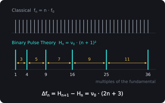
The Recursive Harmonic Spectrum. Classical harmonics sit at whole multiples of the fundamental, fₙ = n · f₀, evenly spaced. Binary Pulse harmonics sit at Hₙ = ν₀ · (n + 1)², at 1, 4, 9, 16, 25 and 36 times ν₀, so the gap between neighbors grows with the harmonic index: Δfₙ = ν₀ · (2n + 3).
The Harmonic Energy Distribution framework demonstrates how Binary Pulse Theory imposes physical constraints on energy allocation across recursive harmonic structures, with the convergence parameter determining whether infinite harmonic series remain physically realizable and providing mathematical boundaries that ensure finite total energy through decay rates faster than quadratic growth in computational substrate architectures.
Convergence Analysis Framework
By analyzing the Convergence Analysis framework, we can understand the mathematical conditions required for finite energy in infinite recursive harmonic series, revealing how convergence parameters determine physical realizability and providing exact numerical solutions through special function analysis for specific parameter values.
Total Energy Convergence
E⊚ = E_0 sum(n=0 to infinity) (n + 1)^(2-γ) [J]
Where:
- E⊚ [𝕄·𝕃²·𝕋⁻²] - total energy across all harmonics
- E_0 [J] - fundamental energy scale
- sum(n=0 to infinity) - infinite summation operator from n=0 (the fundamental, E_n = E_0) to infinity
- n [∅] - harmonic index
- γ [∅] - convergence parameter
- ^(2-γ) [∅] - power law exponent
- infinity [∅] - mathematical limit concept
- [∅] - quantities without physical units, pure numerical ratios or mathematical constants
➢ Series converges when 2-γ < -1, requiring γ > 3 for finite energy systems, establishing fundamental mathematical constraints for physical realizability of infinite recursive harmonic structures in computational substrate architectures.
By examining the specific case where γ = 3.5, we can understand how the Hurwitz Zeta Function provides exact convergent values for total energy in recursive harmonic systems, demonstrating concrete numerical results for physically realizable infinite harmonic series.
Hurwitz Zeta Convergence
E⊚ = E_0 ζ(1.5, 1) ≈ 2.612 E_0 [J]
Where:
- E⊚ [𝕄·𝕃²·𝕋⁻²] - total energy across all harmonics for γ = 3.5
- E_0 [J] - fundamental energy scale
- ζ(s,a) [∅] - Hurwitz Zeta Function with arguments s and a
- s [∅] - first argument, equal to 1.5
- a [∅] - second argument, equal to 1 (the first term of the sum, n + 1 = 1 at n = 0)
- 1.5 [∅] - zeta function parameter s = γ - 2 = 3.5 - 2 = 1.5
- 1 [∅] - zeta function parameter a
- 2.612 [∅] - approximate numerical value of ζ(1.5, 1), which equals the Riemann zeta value ζ(1.5)
- [∅] - quantities without physical units, pure numerical ratios or mathematical constants
➢ Specific convergent value ensuring finite total energy in recursive harmonic systems, demonstrating concrete numerical results for γ = 3.5 case that satisfies convergence requirements.
The Convergence Analysis framework demonstrates how Binary Pulse Theory provides rigorous mathematical foundations for infinite harmonic series through convergence parameter constraints and special function solutions. The general convergence condition γ > 3 ensures finite total energy while the specific γ = 3.5 case illustrates exact numerical evaluation through Hurwitz Zeta functions, establishing both theoretical boundaries and practical computational methods for analyzing energy distribution in recursive harmonic systems within computational substrate architectures.
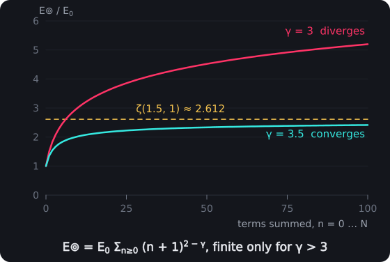
Convergence of the Harmonic Energy. Partial sums of E⊚ = E₀ Σ (n + 1)^(2−γ) from n = 0. At γ = 3.5 the total levels off at E₀ ζ(1.5, 1) ≈ 2.612 E₀; at γ = 3, the edge of the convergence condition γ > 3, it grows without limit.
Spectral Complexity Quantification
Spectral Complexity Measures (G) quantify the computational intricacy embedded in harmonic structures, drawing from information theory approaches in nonlinear dynamics (Strogatz, 2014)²⁴.
By examining the Spectral Complexity Quantification framework, we can understand how information theory metrics quantify computational intricacy in recursive harmonic systems, revealing the mathematical tools for characterizing complexity distribution, recursion depth concentration, and frequency clustering patterns that distinguish Binary Pulse Theory architectures from classical harmonic structures.
Spectral Complexity Index
C⚚ = -sum_n p_n log_2(p_n) [1ᵇ]
Where:
- C⚚ [1ᵇ] - Spectral Complexity Index
- sum_n - summation operator over all harmonic indices n
- p_n [∅] - normalized energy distribution, equal to E_n/E⊚
- log_2 - logarithm base 2 function
- n [∅] - harmonic index
- E_n [J] - energy of nth harmonic
- E⊚ [𝕄·𝕃²·𝕋⁻²] - total energy across all harmonics
- [∅] - quantities without physical units, pure numerical ratios or mathematical constants
➢ Information entropy measures quantifying spectral complexity in harmonic distribution, providing quantitative assessment of information content encoded in energy allocation patterns across recursive frequency structures in computational substrate architectures.
Recursive Depth Indicator
Dℜ = sum_n n² × p_n / sum_n n × p_n [∅]
Where:
- Dℜ [∅] - Recursive Depth Indicator
- sum_n - summation operator over all harmonic indices n
- n [∅] - harmonic index
- p_n [∅] - normalized energy distribution, equal to E_n/E⊚
- [∅] - quantities without physical units, pure numerical ratios or mathematical constants
➢ Weighted average recursion depth measuring computational complexity concentration, providing quantitative assessment of how processing load distributes across recursion levels in harmonic systems with higher values indicating concentration at deeper computational layers.
Harmonic Clustering Coefficient
K⋒ = ⟨|H_(n+1) - H_n|⟩ / ⟨H_n⟩ [∅]
Where:
- K⋒ [∅] - Harmonic Clustering Coefficient
- ⟨ ⟩ - ensemble average operator
- |H_(n+1) - H_n| [𝕋⁻¹] - absolute frequency difference between consecutive harmonics
- H_(n+1) [𝕋⁻¹] - (n+1)th harmonic frequency
- H_n [𝕋⁻¹] - nth harmonic frequency
- n [∅] - harmonic index
- [∅] - quantities without physical units, pure numerical ratios or mathematical constants
➢ Ratio quantifying frequency clustering patterns in recursive harmonic spectra, providing measures of how frequency spacing deviates from uniform distribution and characterizing the clustering effects produced by quadratic frequency scaling in computational substrate architectures.
The Spectral Complexity Quantification framework demonstrates how Binary Pulse Theory integrates information theory with harmonic analysis to provide comprehensive characterization tools for recursive computational systems. The spectral complexity index quantifies information content through entropy measures, the recursive depth indicator reveals computational load concentration patterns, and the harmonic clustering coefficient characterizes frequency distribution deviations, collectively enabling systematic analysis of computational intricacy embedded in harmonic structures and distinguishing recursive substrate architectures from classical uniform systems.
7.1 Testable Predictions
- Quadratic Frequency Scaling: Nonlinear frequency spacing Δf_n = ν_sys × (2n + 3) in quantum dot arrays, with ν_sys the fundamental of the system measured (ν_0 is the substrate case), reflecting computational complexity scaling, measurable via high-resolution spectroscopy.
- Power-Law Energy Distribution: Energy scaling E_n proportional to (n + 1)^(2-γ) with γ ≈ 3.5 in coupled oscillator networks, observable through amplitude measurements.
- Harmonic Clustering: Geometric clustering around f⋒,k = ν_sys × k² in nonlinear optical cavities, detectable via frequency comb analysis.
- Spectral Complexity Scaling: Information entropy C⚚ = -sum_n p_n log_2(p_n) measurements in recursive antenna arrays, quantifiable through signal processing techniques.