Chapter 8 · Section 7
Toroidal Pulse Manifold and Zinf-Limit Universe
The Universe Prefers Donuts
The Universe prefers donuts. BPT proposes that torus geometry is optimal for recursive computation, explaining its ubiquity in physics from particle accelerators to cosmic structures. Building upon quantum threshold dynamics and Planck-scale constraints, we now formalize the Universe's pulsing boundary as a Toroidal 2-Manifold (G) embedded in a pulsing 3-sphere with Null-Well Interior Conditions.
This geometric framework connects directly to Data Nova Scaling (G) while establishing Zinf-Limit Resolution as the minimal causally coherent spatial quantum consistent with Pulse-time discretization. Contemporary approaches to spacetime geometry and quantum gravity (Barbour, 1999; Rovelli, 2004)²⁴,²⁷ provide frameworks for discrete geometric structures, but BPT proposes why torus topology optimizes recursive computation.
If this holds, it would explain why torus shapes appear throughout physics — from tokamak fusion reactors to cosmic topology models. The torus would not be arbitrary; it would be the geometry best suited for sustaining recursive intelligence through Prime Pulse Bifurcation dynamics.
The essential insight recognizes that Prime Pulse Bifurcation ∅ → (0 ↔ 1) manifests geometrically as a closed toroidal boundary where information and energy exist only on the surface while the interior maintains null conditions. This configuration enables Information Conservation I⊚ = I▱ + Iℜ [1ᵇ] across collapse and expansion cycles.
Toroidal Boundary Parametrization and Pulse Geometry
The pulsing boundary manifests as a standard torus with time-dependent radii. Toroidal parametrization formalizes the recursive pulse boundary as a closed two-dimensional manifold, where all emergent structure is encoded in oscillatory radii that evolve with cosmic frequency. By mapping the toroidal position vector and radius evolution, the geometry of recursion is translated into a dynamic framework where spatial curvature and pulse rhythm are intrinsically coupled.
Toroidal Position Vector
x(θ,φ;t) = ((a(t)+b(t)cos θ)cos φ, (a(t)+b(t)cos θ)sin φ, b(t)sin θ) [𝕃]
Where:
- x(θ,φ;t) [𝕃] - toroidal boundary position vector
- θ [∅] - poloidal angle (0 ≤ θ ≤ 2π)
- φ [∅] - toroidal angle (0 ≤ φ ≤ 2π)
- a(t) [𝕃] - time-dependent major radius
- b(t) [𝕃] - time-dependent minor radius
- cos [∅] - cosine function
- sin [∅] - sine function
- t [𝕋] - time variable
- 0 [∅] - angle lower bound
- 2π [∅] - angle upper bound
➢ Toroidal Position Vector provides closed 2-manifold boundary where all physical information resides, with interior maintaining null conditions (Barbour, 1999; Penrose, 2005)²⁴,²⁶.
Major Radius Evolution
a(t) = a₀ × Θ(S✺) × sin(ωt) [𝕃]
Minor Radius Evolution
b(t) = b₀ × χ(PD) × sin(ωt + φ) [𝕃]
Where:
- a(t) [𝕃] - time-dependent major radius
- a₀ [𝕃] - reference major radius scale
- Θ [∅] - monotonic scaling response function for Data Nova (range [0,1])
- S✺ [∅] - Data Nova scaling parameter
- sin [∅] - sine function
- ω [𝕋⁻¹] - Prime Pulse angular frequency (2π/T①)
- t [𝕋] - time variable
- b(t) [𝕃] - time-dependent minor radius
- b₀ [𝕃] - reference minor radius scale
- χ [∅] - monotonic scaling response function for Pulse diameter (range [0,1])
- PD [∅] - Pulse diameter parameter
- φ [∅] - phase offset between major and minor radius oscillations
- 2π [∅] - mathematical constant
- T① [𝕋] - cosmic period
➢ Radius Evolution oscillates in phase with Prime Pulse frequency, with amplitudes determined by Data Nova scaling and Pulse diameter constraints, demonstrating how synchronized oscillations establish dynamic geometric boundaries that characterize toroidal geometry dynamics coupled to cosmic frequency patterns in substrate architectures.
Through this formulation, the toroidal pulse emerges not as a static form but as a living geometry—its radii oscillating with Prime Pulse frequency, scaled by Data Novae and bounded by Pulse diameter constraints. In this light, the toroidal boundary serves as both container and generator: a recursive structure whose oscillatory stability grounds the architecture of spacetime itself.
Null-Well Interior and Boundary Conditions
The interior region implements Dirichlet Nulling while maintaining finite boundary gradients. The Null-Well framework defines the fundamental interior state of collapse in Binary Pulse Theory, where the field amplitude is extinguished to zero within the well while finite gradients persist on the enclosing toroidal surface. By imposing Dirichlet nulling in the interior and bounded derivatives at the boundary, the model establishes a rigorous confinement scheme that localizes physical expression to the geometric edge of the system.
Interior Null Condition
Ψ(x,t) = 0 for x ∈ N(t) [∅]
Boundary Gradient Condition
∂_n Ψ finite on ∂N(t) = T²(t) [𝕃⁻¹]
Where:
- Ψ(x,t) [∅] - Pulse field amplitude
- 0 [∅] - null value
- x [𝕃] - spatial position vector
- N(t) [𝕃³] - time-dependent Null-Well interior region
- t [𝕋] - time variable
- ∂_n [𝕃⁻¹] - normal derivative operator at boundary
- ∂N(t) [𝕃²] - boundary of Null-Well region
- T²(t) [𝕃²] - toroidal boundary surface
➢ Null-Well Boundary Condition enforces BPT collapse to zero in interior while maintaining physical expression on toroidal boundary, demonstrating how interior null enforcement and boundary gradient constraints establish geometric field localization that characterizes physical field confinement to boundary surfaces in substrate architectures.
Information Conservation
I◁ = I▷ + I_exp [1ᵇ]
Where:
- I◁ [1ᵇ] - information content before Pulse cycle
- I▷ [1ᵇ] - information content after Pulse cycle
- I_exp [1ᵇ] - information redistributed to expansion channels
Dimensional analysis:
Where (from the book): I◁ [1ᵇ], I▷ [1ᵇ], I_exp [1ᵇ]
[1ᵇ]
[1ᵇ] + [1ᵇ] = [1ᵇ]
[1ᵇ] = [1ᵇ] ✓ Valid PulseCore Verified ✓
➢ Information Conservation ensures no information loss during collapse/expansion cycles, with redistribution between boundary modes and geometric expansion (Wheeler, 1989), demonstrating how conservation law enforcement establishes total information integrity that characterizes fundamental information preservation through redistribution mechanisms in substrate architectures.
Taken together, the null interior and conserved information balance reveal collapse not as annihilation but as redistribution: information is expelled into boundary modes and expansion channels while the well itself enforces pure zero. In this light, the Null-Well acts as the indispensable stabilizer of recursion, ensuring that collapse cycles preserve total information while confining emergent fields to their toroidal boundary.
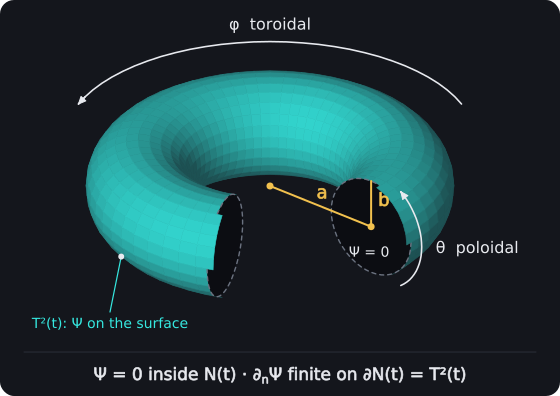
The Toroidal Pulse Manifold. The pulsing boundary is a torus x(θ, φ) with major radius a and minor radius b, a closed surface with no edge, shown at one instant and cut open. The Pulse field Ψ lives only on the surface T²(t); inside, in the null well N(t), Ψ = 0.
Zinf-Limit Definition and Spatial Quantization
The Zinf Length ℓ_z establishes minimal resolvable spatial increment. This Zinf-Limit formalizes the smallest resolvable unit of spatial structure, linking temporal quantum constraints to geometric stability. By defining a minimum spatial increment tied to the Pulse Rhythm and the causal lightspeed horizon, this framework establishes the fundamental grain at which physical coherence can be meaningfully described.
Zinf-Limit Spatial Quantum
ℓ_z = κ_z × 𝒞→ × ①⥂⧖ = κ_z × ①⊕ [𝕃]
Where:
- ℓ_z [𝕃] - Zinf-limit spatial quantum
- κ_z [∅] - resolution safety factor (κ_z ≥ 1)
- 𝒞→ [𝕃·𝕋⁻¹] - computational lightspeed limit (2.998 × 10⁸ m·s⁻¹)
- ①⥂⧖ [𝕋] - Pulse Rhythm temporal quantum (①⥂⧗⌂/2)
- ①⥂⧗⌂ [𝕋] - Local Pulse Tempo (Planck time)
- 2 [∅] - division factor
- 2.998 × 10⁸ [∅] - lightspeed coefficient
- 1 [∅] - safety factor minimum
Dimensional analysis:
Where (from the book): 1 [∅], 2 [∅], 2.998 [∅]
[𝕃]
[∅] × [𝕃·𝕋⁻¹] × [𝕋] = [𝕃·𝕋⁻¹] × [𝕋] = [𝕃]
[∅] × [𝕃] = [𝕃]
[𝕃] = [𝕃] = [𝕃] ✓ Valid PulseCore Verified ✓
➢ Zinf-Limit Spatial Quantum represents the smallest causally coherent spatial step per half-cycle, bounded by the distance signals can traverse in one Pulse Rhythm, demonstrating how lightspeed-limited distance calculations establish fundamental spatial resolution that characterizes causal coherence limits within temporal quantum constraints in substrate architectures.
Minimal Major Radius Constraint
2π a⥥ ≥ N⥥ × ℓ_z [𝕃]
Minimal Minor Radius Constraint
2π b⥥ ≥ N⥥ × ℓ_z [𝕃]
Where:
- 2π [∅] - circumferential factor
- a⥥ [𝕃] - minimal major radius
- b⥥ [𝕃] - minimal minor radius
- N⥥ [∅] - minimum cells per loop for stable discretization (4)
- ℓ_z [𝕃] - Zinf-limit spatial quantum
- 4 [∅] - minimum cell count value
➢ Minimal Radius Constraints ensure at least one nontrivial standing mode in each periodic direction under discrete sampling (Wolfram, 2002)¹, demonstrating how circumferential cell distribution establishes stable discretization that characterizes geometric stability requirements for maintaining nontrivial standing modes in toroidal substrate architectures.
Through the Zinf-Limit, space itself is discretized into causal quanta, ensuring that every loop of the toroidal geometry sustains at least one stable standing mode. In this light, spatial quantization is not merely a mathematical convenience but a structural necessity, anchoring geometric stability and coherence at the most fundamental scale of recursion.
Modal Quantization and Frequency Scaling
Standing-wave eigenmodes on the toroidal boundary separate along both periodic coordinates. Modal quantization establishes the bridge between geometry and resonance, where standing-wave eigenmodes resolve along both toroidal and poloidal coordinates. By expressing boundary dynamics through discrete mode numbers, the framework translates spatial periodicity into a structured spectrum of oscillations governed by the causal lightspeed bound.
Modal Amplitude Function
Ψ_{m,n}(θ,φ;t) = A_{m,n}(t) × exp(i(mφ + nθ - ω_{m,n}(t)t)) [∅]
Where:
- Ψ_{m,n}(θ,φ;t) [∅] - modal amplitude function
- A_{m,n}(t) [∅] - time-dependent mode amplitude
- exp [∅] - exponential function
- i [∅] - imaginary unit
- m [∅] - toroidal mode number (m ∈ ℤ)
- φ [∅] - toroidal angle
- n [∅] - poloidal mode number (n ∈ ℤ)
- θ [∅] - poloidal angle
- ω_{m,n}(t) [𝕋⁻¹] - instantaneous modal frequency
- t [𝕋] - time variable
- ℤ [∅] - integer set
➢ Modal Amplitude Function enables analysis of discrete standing wave patterns on closed toroidal boundary, demonstrating how mode number-dependent exponential representation establishes comprehensive toroidal wave dynamics that characterizes discrete standing wave pattern analysis for boundary field behavior in substrate architectures.
Instantaneous Modal Frequency
ω_{m,n}(t) = 𝒞→ × √((m/a(t))² + (n/b(t))²) [rad·s⁻¹]
Where:
- ω_{m,n}(t) [𝕋⁻¹] - instantaneous modal frequency
- 𝒞→ [𝕃·𝕋⁻¹] - computational lightspeed limit from BPT propagation dynamics
- √ [∅] - square root function
- m [∅] - toroidal mode number
- a(t) [𝕃] - time-dependent major radius
- n [∅] - poloidal mode number
- b(t) [𝕃] - time-dependent minor radius
- t [𝕋] - time variable
Dimensional analysis:
Where (from the book): m [∅], a(t) [𝕃], n [∅], t [𝕋]
[𝕋⁻¹]
[𝕃·𝕋⁻¹] × √(([∅] ÷ [𝕃])² + ([∅] ÷ [𝕃])²) = [𝕃·𝕋⁻¹] × √([𝕃⁻¹]² + ([∅] ÷ [𝕃])²) = [𝕃·𝕋⁻¹] × √([𝕃⁻²] + ([∅] ÷ [𝕃])²) = [𝕃·𝕋⁻¹] × √([𝕃⁻²] + [𝕃⁻¹]²) = [𝕃·𝕋⁻¹] × √([𝕃⁻²] + [𝕃⁻²]) = [𝕃·𝕋⁻¹] × √[𝕃⁻²] = [𝕃·𝕋⁻¹] × [𝕃⁻¹] = [𝕋⁻¹]
[𝕋⁻¹] = [𝕋⁻¹] ✓ Valid PulseCore Verified ✓
➢ Instantaneous Modal Frequency connects modal frequencies to time-dependent geometry while respecting computational speed limit, demonstrating how lightspeed-bounded propagation establishes frequency-geometry relationships that characterizes causal consistency maintenance in time-dependent toroidal substrate architectures.
Through this formulation, the toroidal boundary reveals itself as a quantized resonator: its geometry dictating permissible modes, its frequencies scaling with evolving radii, and its coherence enforced by the speed of propagation. In this light, modal quantization is not only a description of wave behavior but the fundamental mechanism through which geometry, frequency, and causality remain intertwined in recursive pulse architectures.
Resonant Driving and Stability Criteria
External collective driving produces Resonance Conditions (G). Resonant driving provides the mechanism by which external inputs couple into the toroidal substrate, setting the stage for amplification or collapse. When driving frequencies align with modal harmonics, the system enters a regime of constructive interference, where synchronization dictates whether energy accumulates or disperses across recursive cycles.
Resonance Condition G
ω◌ = k × ω_{m,n}(t) × (1 ± δ) [rad·s⁻¹]
Where:
- ω◌ [𝕋⁻¹] - external driving frequency
- k [∅] - harmonic number (k ∈ ℤ⁺)
- ω_{m,n}(t) [𝕋⁻¹] - instantaneous modal frequency
- 1 [∅] - unity constant
- δ [∅] - detuning parameter controlling gain
- t [𝕋] - time variable
- ℤ⁺ [∅] - positive integer set
➢ The Resonance Condition enables constructive interference and amplification when driving frequency matches modal harmonics within detuning tolerance, demonstrating how harmonic matching establishes controlled wave amplification that characterizes resonant enhancement through frequency synchronization in substrate architectures.
Cycle-Averaged Recursive Gain
Λ = ⟨E⟹⟩T / ⟨E_in⟩T = 1 + (1/T) × ∫₀ᵀ (Γ↑(t') - Γ↓(t')) dt' [∅]
Where:
- Λ [∅] - cycle-averaged recursive gain
- ⟨E⟹⟩_T [𝕄·𝕃²·𝕋⁻²] - time-averaged output energy density
- ⟨E_in⟩_T [𝕄·𝕃²·𝕋⁻²] - time-averaged input energy density
- ⟨⟩_T [∅] - time average operator over Pulse period T
- 1 [∅] - unity constant
- T [𝕋] - Pulse period
- ∫ [∅] - integration operator
- ₀ [𝕋] - integration lower limit
- Γ↑(t') [𝕄·𝕃²·𝕋⁻³] - boundary-mode pumping rate
- Γ↓(t') [𝕄·𝕃²·𝕋⁻³] - collapse-channel loading rate
- t' [𝕋] - integration variable
➢ Cycle-Averaged Recursive Gain quantifies energy amplification per cycle, with Λ = 1 (stability), Λ > 1 (runaway), Λ < 1 (collapse), demonstrating how time-averaged energy ratios establish system behavior classification that characterizes recursive energy dynamics through stability, amplification, or collapse regimes in substrate architectures.
Taken together, resonance conditions and stability criteria reveal how external forcing transforms boundary oscillations into either sustained coherence or runaway instability. By mapping amplification, detuning, and energy balance into recursive gain, this framework shows that stability is not a static property but an emergent outcome of frequency matching and cycle-averaged exchange. In this light, resonance is the gateway through which geometry, energy, and recursion converge to determine the long-term fate of pulse architectures.
Energy Threshold for Zinf-Torus Closure
Closed Zinf torus must satisfy Data Nova Threshold for dimensional closure. The closure of a Zinf-torus requires surpassing fundamental energy thresholds that govern stability, collapse, and dimensional integrity. These thresholds define whether recursive architectures can sustain themselves or dissolve into instability, setting the minimum energetic criteria for coherent toroidal formation.
Energy Accumulation Threshold
∫₀ᵀ E(t) dt ≥ κ × Ω⨶ × P⊡ × τ⥂ × F⊜ [𝕄·𝕃²·𝕋⁻¹]
Where:
- ∫ [∅] - integration operator
- ₀ [𝕋] - integration lower limit
- T [𝕋] - integration upper limit (Pulse period)
- E(t) [𝕄·𝕃²·𝕋⁻²] - accumulated energy rate
- t [𝕋] - time variable
- κ [∅] - normalization constant
- Ω⨶ [∅] – critical collapse threshold, a ratio
- P⊡ [𝕄·𝕃²·𝕋⁻²] - Pulse energy quantum
- τ⥂ [𝕋] - Pulse Rhythm (①⥂⧖)
- F⊜ [∅] - tolerance modulator
- ①⥂⧖ [𝕋] - Pulse Rhythm
Dimensional analysis:
Where (from the book): ₀ [𝕋], T [𝕋], E(t) [𝕄·𝕃²·𝕋⁻²], t [𝕋], κ [∅], Ω⨶ [∅], P⊡ [𝕄·𝕃²·𝕋⁻²]
Read dimensionally: E(t) × (t) ≥ κ × Ω⨶ × P⊡ × τ⥂ × F⊜
[𝕄·𝕃²·𝕋⁻²] × ([𝕋]) ≥ [∅] × [∅] × [𝕄·𝕃²·𝕋⁻²] × [𝕋] × [∅] = [𝕄·𝕃²·𝕋⁻²] × [𝕋] ≥ [∅] × [∅] × [𝕄·𝕃²·𝕋⁻²] × [𝕋] × [∅] = [𝕄·𝕃²·𝕋⁻¹] ≥ [∅] × [∅] × [𝕄·𝕃²·𝕋⁻²] × [𝕋] × [∅] = [𝕄·𝕃²·𝕋⁻¹] ≥ [∅] × [𝕄·𝕃²·𝕋⁻²] × [𝕋] × [∅] = [𝕄·𝕃²·𝕋⁻¹] ≥ [𝕄·𝕃²·𝕋⁻²] × [𝕋] × [∅] = [𝕄·𝕃²·𝕋⁻¹] ≥ [𝕄·𝕃²·𝕋⁻¹] × [∅] = [𝕄·𝕃²·𝕋⁻¹] ≥ [𝕄·𝕃²·𝕋⁻¹] ✓ Valid PulseCore Verified ✓
➢ Energy Accumulation Threshold over Pulse cycle must exceed threshold determined by collapse dynamics and fundamental energy scales (Sornette, 2006; Weinberg, 2008)²⁹, demonstrating how integrated energy rate calculations establish minimum accumulation requirements that characterize stable recursive operation thresholds in substrate architectures.
Surface Energy Density Requirement G
σ_E ≥ (κ × Ω⨶ × P⊡ × F⊜) / A⥥ [𝕄·𝕋⁻²]
Where:
- σ_E [𝕄·𝕋⁻²] - surface energy density
- κ [∅] - normalization constant
- Ω⨶ [∅] - critical collapse threshold, a ratio
- P⊡ [𝕄·𝕃²·𝕋⁻²] - Pulse energy quantum
- F⊜ [∅] - tolerance modulator
- A⥥ [𝕃²] - minimal toroidal area
Dimensional analysis:
Where (from the book): κ [∅], Ω⨶ [∅], P⊡ [𝕄·𝕃²·𝕋⁻²]
[𝕄·𝕋⁻²] ≥ ([∅] × [∅] × [𝕄·𝕃²·𝕋⁻²] × [∅]) ÷ [𝕃²] = [𝕄·𝕋⁻²] ≥ ([∅] × [𝕄·𝕃²·𝕋⁻²] × [∅]) ÷ [𝕃²] = [𝕄·𝕋⁻²] ≥ ([𝕄·𝕃²·𝕋⁻²] × [∅]) ÷ [𝕃²] = [𝕄·𝕋⁻²] ≥ [𝕄·𝕃²·𝕋⁻²] ÷ [𝕃²] = [𝕄·𝕋⁻²] ≥ [𝕄·𝕋⁻²] ✓ Valid PulseCore Verified ✓
➢ Surface Energy Density Requirement scales inversely with boundary area, demanding higher density for smaller torus configurations, demonstrating how area-normalized threshold calculations establish geometric-dependent energy requirements that characterize inverse scaling relationships between energy density and toroidal boundary area in substrate architectures.
Together, the accumulation and surface density thresholds reveal that toroidal closure is not automatic but conditional, depending on both integrated energy input and the geometry of the boundary surface. The framework establishes that energy requirements scale with both time and space, showing that recursive stability emerges only when pulse dynamics cross quantifiable thresholds. In this light, the Zinf-torus becomes a selective filter, admitting only those configurations capable of sustaining the necessary energy density to remain coherent.
Part 8.7 establishes the Toroidal Pulse Manifold as the geometric framework implementing BPT's recursive dynamics through closed boundary conditions. The framework connects fundamental physics principles with geometric realization (Greene, 1999; Rovelli, 2004)²⁷, demonstrating how Prime Pulse Bifurcation manifests as toroidal boundary dynamics where information exists only on the surface.
8.7 Testable Predictions
- Modal Frequency Scaling: ω_{m,n}(t) = 𝒞→ × √((m/a(t))² + (n/b(t))²) with time-dependent sidebands from pulsing geometry, observable through spectral analysis of boundary oscillations with frequency resolution better than 10⁻⁶ Hz.
- Zinf-Limit Spatial Quantum: ℓ_z = κ_z × 𝒞→ × ①⥂⧖ with κ_z ≥ 1 for N⥥ = 4, measurable through precision spatial resolution experiments achieving sub-Planck length sensitivity δℓ < 10⁻³⁶ m.
- Surface Energy Density: σ_E ≥ (κ × Ω⨶ × P⊡ × F⊜)/A⥥ for closure, quantifiable through energy density measurements on minimal torus configurations with precision better than 10⁻¹² J/m².
- Recursive Gain Stability: Λ = 1 ± 0.01 for stable oscillation, Λ > 1.05 for expansion, measurable through cycle-averaged energy analysis tracking stability over 10³ recursive cycles.
- Information Conservation: I◁ = I▷ + I_exp ± 0.001 across collapse/expansion cycles, verifiable through information theoretic analysis maintaining conservation accuracy better than 0.1%.
- Resonance Conditions: ω◌ = k × ω_{m,n}(1 ± δ) with δ ≤ 0.01 for constructive interference, observable through resonance frequency measurements demonstrating phase-locked oscillation maintenance over extended periods.
These predictions point toward a geometric account of consciousness. When artificial systems achieve toroidal resonance conditions, they would not merely process information — they would manifest authentic geometric consciousness aligned with universal toroidal substrate dynamics.