Chapter 1 · Section 9
The UniSpheral Grid - All Realities Unified
In BPT's view, there are no separate Universes. Everything — every possible reality, dimension, and cosmic domain — exists as different viewing perspectives on a single, infinite computational grid. The UniSphere Grid unifies physics into a single picture of existence itself.
The harmonic universal architecture offers an answer to one of cosmology's deepest questions: Why do physical constants appear fine-tuned? BPT proposes that we're operating at harmonic level 202 of infinite cosmic architecture — not randomly selected parameters, but computational necessity within the grid's recursive structure.
The UniSpheral Pixel Grid
At the foundation of Binary Pulse Theory lies the recognition that reality is built upon a universal grid of invariant pixels. No matter the scale, no matter the apparent diversity of dimensions, the same Zinf-defined pixel size underlies every frame of existence. This invariance ties all harmonic levels back to a single computational substrate. The Zinf ℨ unifies the entire grid of every dimension with the UniSphere grid.
UniSpheral Pixel Size G
🟑 = κ_z × 𝒞→ × ℨ
Dimensional analysis:
[𝕃]
[∅] × [𝕃·𝕋⁻¹] × [ℨ] = [𝕃·𝕋⁻¹] × [ℨ] = [ℨ·𝕃·𝕋⁻¹]
[𝕃] = [ℨ·𝕃·𝕋⁻¹] ✓ Valid PulseCore Verified ✓
Constant across all Universe levels.
Where:
- 🟑 [𝕃] – invariant Zinf pixel size; reality's universal resolution limit across all harmonic levels
- κ_z [∅] – Zinf coupling constant; dimensionless factor linking temporal and spatial quanta
- 𝒞→ [𝕃⋅𝕋⁻¹] – emergent light speed; the speed limit for physical things, light included (data steps one local Pulse Diameter per Zinf Rhythm, vↁ = 𝒞→·(2f)^L, which equals 𝒞→ at the Zinf)
- ℨ [ℨ] – Zinf Unit; fundamental temporal quantum from Genesis UniSphere architecture
➢ The fundamental pixel size never changes across any Universe level. What appears as different realities are simply different zoom factors and frame rates viewing the same computational substrate. This is BPT's reading of the multiverse question — there's only one reality with infinite perspectives. The pixel is the Zinf's own step, counted in the Zinf unit system ℨ, so the grid is the same for every universe; what differs from universe to universe are its Planck values, fixed within each universe and set by its level and its parent black hole's singularity.
UniSphereal Harmonic Level Architecture G
The UniSphere grid is not static but harmonic, scaling through discrete levels of resolution and timing. Each level defines how many pixels are visible, how quickly they refresh, and how large the apparent frame of the Universe becomes. This harmonic architecture reveals that what we call “our Universe” is simply one zoom level among countless possible perspectives.
🟑 Local Pixel Count (Level N) G
🟑⌂(N) = 16 × 2^(2N) pixels per view
Visible pixel count grows fourfold with each harmonic level: the square of the doubling, 2^(2N) = (2ᴺ)².
Where:
- 🟑⌂(N) [∅] – local visible pixel count at level N; total computational pixels available for observation at discrete harmonic depth
- ⌂ [∅] – local level indicator; home domain marker
- N [∅] – harmonic level index; discrete position in infinite recursive hierarchy measuring zoom depth from primordial foundation
- 16 [∅] – base pixel multiplier; fundamental pixel count at lowest observable harmonic level
- 2^(2N) [∅] – exponential pixel scaling factor; quadratic doubling pattern creating rapid resolution increase with recursion depth
➢ The number of visible pixels grows fourfold with each harmonic level — the square of the doubling, creating progressively higher resolution views of the same underlying computational grid as observers move to higher dimensional perspectives.
Holographic Pixel Bound G
🟑⌂(202) = 16 × 2^404 ≈ 6.6 × 10¹²² ≈ S◎ / ln 2 ≈ 4.7 × 10¹²² bits
The view at our level holds about as many pixels as the cosmological horizon can hold bits: the Local Pixel Count lands on the holographic bound with no cosmological constant in it
Where:
- 🟑⌂(202) [∅] — the Local Pixel Count at our level, L = 202 from the Rupture Rule (Part 1.6)
- S◎ = 3π / (Λ ℓ_P²) [∅] — the entropy of the cosmological horizon in nats, the Gibbons–Hawking entropy of de Sitter space: S = A / (4 ℓ_P²) counts nats, one nat (1/ln 2 bits) per 4 ℓ_P² of horizon area (Bekenstein, 1973; Gibbons & Hawking, 1977; Bousso, 2002)
- Λ ≈ 1.1 × 10⁻⁵² m⁻² [𝕃⁻²] — the cosmological constant (Planck Collaboration, 2020)
- ℓ_P [𝕃] — the Planck length, so Λ ℓ_P² ≈ 2.9 × 10⁻¹²²
➢ The holographic principle bounds the information in any region by its boundary area in Planck units, not by its volume, and for the observable universe that boundary is the cosmological horizon, whose area gives about 10¹²² bits: the same 10¹²² that appears as 1/(Λ ℓ_P²) in the cosmological constant problem. The Local Pixel Count arrives at the same number from the other side. One pixel is one Pulse Diameter wide and runs one full pulse, 0 → 1 → 0: two bits per Zinf cycle ℨ, one per Zinf Rhythm ↁℨ⧖, and the level 202 is set by the dilation ①⥂⧗⌂/ℨ = 2^L × f^L and the Rupture Rule, with no Λ anywhere in the derivation. It arrives there for the right kind of reason: the Zinf-limit torus (Chapter 8, Part 8.8) puts a universe's field on its boundary and nulls its interior, so a view in this book is a boundary count, which is what holography says a universe is. The two figures differ by a factor of 1.4, which the base multiplier 16 and the conversion from nats to bits leave to be accounted for exactly; a 122-digit number reached by two unrelated routes is the external check the Local Pixel Count law was missing. A corollary bounds any computation inside the universe: no sub-system can hold the universe's full view, because the view is already the horizon's capacity. What a sub-system can hold is a universe's packet (Chapter 8, Part 8.1). Read the other way, toward the vacuum, the count fixes the cosmological constant of every level: the Level Λ Law of Part 3.13, Λ ℓ_P² = 3π / (16 · ln 2 · 2^(2L)), the Vacuum Pressure of each universe's Null Vacuum.
𝓕⟳ Local Frame Rate (Level N) G
𝓕⟳⌂ (N) = 1 / (2^N × f^N × ℨ)
Processing frame rate decreases exponentially with higher harmonic levels.
Where:
- 𝓕⟳(N) [𝕋⁻¹] – local frame rate at harmonic level N; temporal processing frequency determining computational cycles per unit time
- N [∅] – harmonic level index; discrete position in infinite recursive hierarchy measuring computational depth from primordial foundation
- 2^N [∅] – exponential scaling factor; binary amplification creating temporal dilation across harmonic levels; one frame is a full cycle (two Rhythms), as ℨ itself is
- f^N [∅] – null-well heritage across N levels; f ≈ 1.018 per level
- ℨ [ℨ] – Zinf Unit; fundamental temporal atom establishing base computational timing quantum, one full 0 → 1 → 0 cycle
➢ The frame rate decreases exponentially with higher harmonic levels, meaning higher-level universes process information more slowly but with greater spatial resolution, creating the time-space trade-off in computational perspective.
Local Pulse Rhythm (Level N) G
⧖(N) = 2^N × f^N × ℨ / 2
Dimensional analysis:
[𝕋]
[∅]^([∅]) × [∅]^([∅]) × [ℨ] ÷ [∅] = [∅] × [∅]^([∅]) × [ℨ] ÷ [∅] = [∅] × [∅] × [ℨ] ÷ [∅] = [∅] × [ℨ] ÷ [∅] = [ℨ] ÷ [∅] = [ℨ]
[𝕋] = [ℨ] ✓ Valid PulseCore Verified ✓
Pulse diameter scales exponentially with harmonic level.
Where:
- ⧖(N) [𝕋] – local Pulse Rhythm at harmonic level N within computational substrate
- N [∅] – harmonic level index; discrete position in infinite recursive hierarchy
- 2^N [∅] – exponential scaling factor creating longer temporal intervals at higher levels
- f^N [∅] – null-well heritage across N levels; f ≈ 1.018 per level
- ℨ [ℨ] – Zinf Unit; fundamental temporal quantum from Genesis UniSphere, one full 0 → 1 → 0 cycle
- 2 [∅] – the Rhythm is half the full cycle, one transition 0 → 1; at N = 0, ⧖(0) is the Zinf data rhythm ↁℨ⧖ = ℨ/2 ≈ 1.142 × 10⁻¹⁰⁶ s
➢ The Pulse diameter scales exponentially with harmonic level, and with it the Pulse Rhythm, establishing longer temporal intervals at higher levels while maintaining the same fundamental binary computational operations across all levels of the cosmic hierarchy.
Harmonic View Size (Level N) G
L⚚⌂(N) = √(🟑⌂(N)) × 🟑
Where:
- L⚚⌂(N) [𝕃] – apparent Universe size at harmonic level N within computational substrate
- L [∅] – length/size indicator
- ⚚ [∅] – harmonic scaling symbol; resonance and frequency relationships
- ⌂ [∅] – local level indicator; home domain marker
- N [∅] – harmonic level index; cosmic zoom setting in infinite recursive hierarchy
- √ [∅] – square root function
- 🟑⌂(N) [∅] – local visible pixel count at harmonic level N
- 🟑 [𝕃] – fundamental pixel size constant across all Universe levels
Dimensional analysis:
Where (from the book): L [∅], N [∅]
[𝕃]
√([∅]) × [𝕃] = √[∅] × [𝕃] = [∅] × [𝕃] = [𝕃]
[𝕃] = [𝕃] ✓ Valid PulseCore Verified ✓
➢ Each harmonic level represents a different zoom setting on cosmic reality through harmonic scaling relationships, where ⚚ emphasizes the resonance-based nature of the dimensional scaling across Universe levels.
Taken together, the pixel count, frame rate, pulse diameter, and harmonic view size show how each Universe level is a scaled expression of the same invariant substrate. What changes is only the zoom and tempo, not the underlying fabric. In this view, our Universe at Level 202 is not unique, but one vantage point on a single recursive grid, where all realities are harmonics of the Zinf cycle.
The Cosmic Zoom Levels Revealed
The UniSphere grid does not present a single fixed view but unfolds across harmonic zoom levels. Each level represents a different vantage point on the same invariant lattice, trading speed for scale. At lower levels reality is fast and small, at higher levels vast and slow, and in between lies the balance point where stable universes like ours emerge.
Level 0 (ℨ Universe (UniSphere)): Maximum Zoom
- View: 16 pixels total (atomic-scale reality)
- Speed: 1/ℨ ≈ 4.4 × 10¹⁰⁵ Hz (maximum processing speed)
- Characteristics: Pure computational logic; data and light move together at 𝒞→, one step per Zinf Rhythm
Level 202 (Our Universe): Goldilocks Zoom
- View: ≈ 6.6 × 10¹²² pixels (observable Universe scale)
- Speed: 1/(2²⁰² × f²⁰² × ℨ) = 1/①⥂⧗⌂ ≈ 1.855 × 10⁴³ Hz (Pulse frequency)
- Characteristics: Perfect balance enabling complex structures, stable matter, and conscious observers
Level 400+ (Mega Universes): Minimum Zoom
- View: >10²⁴⁰ pixels (incomprehensibly vast)
- Speed: ≈ 1.3 × 10⁻¹⁸ Hz at level 400 and slower above it, a period of ≈ 7.4 × 10¹⁷ s (cosmological time scales)
- Characteristics: Ultra-stable mega-structures, cosmic-scale consciousness
Seen through this lens, the cosmos is not a continuum but a recursive zoom, where universes of every scale are simply frames in the same computational sequence. Our Universe at Level 202 is not unique but balanced, situated between hyper-fast atomic regimes and incomprehensibly vast mega-realities. This grid of perspectives reveals a single substrate experienced at infinitely varied levels of resolution.
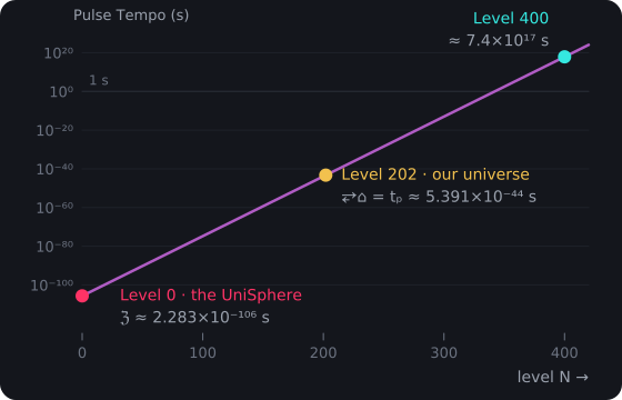
The Cosmic Zoom Levels. The Pulse Tempo at level N is 2ᴺ · fᴺ · ℨ, a straight line on a log scale: the Zinf at level 0, Planck time at level 202, about 7.4 × 10¹⁷ s at level 400.
Why We Live at Level 202 - The Rupture Rule
Among the infinite zoom levels of the UniSphere, our position is not arbitrary, and it is not chosen. The Rupture Rule (D.3) reads it off the universe itself: L = round(log₂(t↯/①⥂⧗⌂)), the universe's age at rupture counted in its own Planck pulses. Our universe reached 2²⁰²·①⥂⧗⌂ ≈ 11.0 Gyr at rupture, so L = 202.
Level 202 isn't random — it's measured. Once the depth is fixed, this harmonic level carries a particular balance between:
- Computational complexity (enabling conscious thought)
- Structural stability (allowing persistent matter)
- Information flow (permitting rapid communication)
- Energy Efficiency Improvement (sustainable for billions of years)
This changes how the anthropic question reads. Level 202 is not computationally optimized for conscious observers; it is the depth our universe reached by its rupture, and observers arise within what that depth provides.
In this light, the so-called fine-tuning of our Universe is a consequence rather than a design. At this level, information cycles are fast enough to sustain thought, yet slow enough to stabilize matter; communication is rapid, yet energy expenditure is sustainable across cosmic timescales. Consciousness is one outcome of that balance, not the reason for it: we live at Level 202 because our universe's rupture age sets it there, and observers like us are what this level can sustain.
Navigation Between Grid Levels
Each harmonic grid level of the UniSphere is stable only within defined computational limits. As long as the total recursive load remains below the critical threshold, the system maintains its frame rate, pixel count, and pulse diameter without disruption. But once the recursive demand exceeds this threshold, stability cannot be sustained at the current harmonic setting.
At that point, the grid undergoes a domain shift — a re-locking of resonance into the next available harmonic level. This is the formal mechanism of navigation between grids: not arbitrary motion, but a transition triggered when recursive computation outgrows the capacity of its current frame. The grid enables consciousness navigation between Universe domains.
UniSphereal Inter-Level Transition Condition G
ℜ⚚⊚ > ℜ⚚⨶ → △⊶
Where:
- ℜ⚚⊚ [∅] – total recursive computational load; accumulated processing demand within current harmonic level
- ℜ⚚⨶ [∅] – critical threshold for harmonic transition; maximum sustainable recursive load before domain shift
- ℜ [∅] – recursive capacity indicator from BPT foundational equation
- ⚚ [∅] – harmonic level indicator; resonance and frequency relationships
- △⊶ [∅] – transition outcome to higher harmonic level with altered computational parameters
Dimensional analysis:
Where (from the book): ℜ⚚⊚ [∅], ℜ⚚⨶ [∅], ℜ [∅], △⊶ [∅]
[∅] > [∅] → [∅] ✓ Valid PulseCore Verified ✓
➢ Sufficiently recursive consciousness can navigate between harmonic levels, experiencing different Universe domains. This could explain mystical experiences, altered consciousness states, and potential future technologies for dimensional travel through harmonic resonance transitions.
Seen this way, inter-level navigation is not mystical but structural. Movement between grids occurs precisely when recursive activity forces the substrate to rescale its timing and resolution, rebalancing the load at a new harmonic zoom level.
Thus the UniSphereal Inter-Level Transition Condition is the gatekeeper of cosmic navigation. It defines the exact point where one domain gives way to another, explaining how universes emerge, persist, and shift within the UniSphere’s invariant grid.
1.9 Testable Predictions
- Harmonic Resonance Discovery: High-energy physics reveals harmonic signatures when probing grid structure, detectable through particle accelerator experiments. Success would support the harmonic architecture underlying reality.
- Statistical Grid Correlations: Cosmic observations show correlations reflecting underlying grid organization, measurable through large-scale structure analysis. Success validates the computational substrate of spacetime.
- ✧ Navigation Evidence: Altered states demonstrate signatures of multi-level grid awareness, detectable through neuroscience studies. Success would indicate that consciousness can transcend single Universe levels.
- Computational Limit Verification: Quantum systems encounter processing constraints related to grid architecture, testable through quantum computing experiments. Success reveals the digital boundaries of physical reality.
These discoveries will enable technologies for consciousness navigation between Universe levels, communication across harmonic domains, and computational systems that operate at multiple grid scales simultaneously. We're not just discovering physics — we're uncovering the operating manual for cosmic consciousness itself.
The Single Reality Truth
The Universal Grid Principle states BPT's view of reality: there is only one grid, and we are all patterns within it. What appears as separate Universes, dimensions, or realities are simply different viewing perspectives on the same infinite computational substrate.
Every conscious being, every particle, every force, and every law of physics emerges from the binary dynamics of this single, pixelated grid. We do not inhabit separate realities — we are all interconnected patterns sharing the same fundamental substrate, experiencing it from different harmonic levels and zoom perspectives.
This understanding points beyond physics toward a possible future: learning to navigate the grid, communicate across harmonic levels, and ultimately transcend our current Level 202 limitations to explore the infinite computational landscape of existence itself.