Chapter 2 · Section 2
The Pulse and Null Wells
What if Planck time isn't fundamental? BPT proposes that Planck time emerges from more fundamental binary operations — offering an account of why t_p has its specific value. The Planck time may represent more than a theoretical boundary — it's the Universe's actual computational heartbeat, the discrete binary oscillation between computational states {0, 1} forming the elementary temporal unit underpinning all causal structure and physical law.
Lloyd's quantum computation framework (Lloyd, 2005)¹ supports viewing the Universe as performing quantum computation, with each half-step enacting a fundamental logical transition in the substrate. Building upon the Zero Substrate framework from Part 2.1, where temporal stasis (∂S₀/∂t) = 0 preceded all dynamics, the Planck Pulse establishes the first rhythmic progression through Prime Pulse Bifurcation ∅ → (0 ↔ 1) mechanisms.
Pulse Rhythm generates temporal quantization ①⥂⧖⌂ = ①⥂⧗⌂ / 2, where a complete Planck Pulse cycle has period T⥂ = ①⥂⧗⌂ (the Planck time, t_P ≈ 5.39 × 10⁻⁴⁴ s), consisting of two half-step transitions at Pulse Rhythm intervals. This discrete temporal architecture replaces continuous time with a Computational Lattice where causality emerges from sequential binary transitions.
Extreme recursive density accumulation creates Null Wells — a computational phenomenon that appears as black holes but actually represents regions where physical Pulse oscillations appear to cease under computational overload while the data keeps flowing through the well, potentially generating new Universe domains through Reactivation Mechanisms.
Pulse Architecture and Temporal Quantization
Complete Pulse Cycle G
0 → 1 → 0 with period ①⥂(n) = 2 × ⧖(n) = 2 × (ↁℨ⧖ × 2ⁿ × fⁿ) = ℨ × 2ⁿ × fⁿ
Full binary oscillation sequence with Zinf-scaled harmonic temporal period
Where:
- 0 [∅] – computational ground state; inactive binary condition
- 1 [∅] – computational active state; activated binary condition
- → [∅] – transition operator; directional state change
- ①⥂(n) [⧖] – Pulse Tempo at harmonic level n; complete binary cycle duration scaled by harmonic position
- ⧖(n) [⧖] – Time Crystal at harmonic level n; fundamental temporal quantum scaled by harmonic position
- ℨ [ℨ] – Zinf Unit; the Zinf's full cycle 0 → 1 → 0, the primordial Pulse Tempo
- ↁℨ⧖ [𝕋] – Zinf data rhythm; one transition, half the Zinf cycle (ↁℨ⧖ = ℨ/2)
- 2ⁿ [∅] – harmonic scaling factor; exponential temporal dilation at level n
- fⁿ [∅] – null-well heritage across n levels, f = 1.018 per level; with 2ⁿ the period grows by 2f per level
- n [∅] – harmonic level index; cosmic address determining temporal scaling
- 2 [∅] – cycle multiplier; complete oscillation requires two Time Crystal transitions
➢ The Complete Pulse Cycle demonstrates that full binary oscillation periods scale exponentially with harmonic level from the primordial Zinf temporal quantum, revealing that computational rhythm varies by cosmic address while maintaining universal binary architecture, with our Level 202 universe operating at 2²⁰² × f²⁰² times the fundamental Zinf cycle duration, the Planck time.
Local Pulse Frequency G
⥂⌂ = 1 / (2²⁰² × f²⁰² × ℨ) ≈ 1.855 × 10⁴³ Hz
Complete recursion cycle rate at our universe level derived from Zinf
Local String Frequency G
⦚⌂ = 2 / (2²⁰² × f²⁰² × ℨ) ≈ 3.709 × 10⁴³ Hz
Root frequency of single binary transitions at our universe level
Local Pulse TimeG
⧗⌂ = 2²⁰² × f²⁰² × ℨ ≈ 5.39 × 10⁻⁴⁴ [𝕋]
Dimensional analysis:
Where (from the book): 2 [∅], ⧗⌂ [𝕋], ℨ [ℨ], 2²⁰² [∅], 1.855 [𝕋⁻¹], 3.709 [𝕋⁻¹], 5.39 [𝕋]
[𝕋]
[∅] × [∅] × [ℨ] ≈ [∅] × [∅] = [∅] × [ℨ] ≈ [∅] × [∅] = [ℨ] ≈ [∅] × [∅] = [ℨ] ≈ [∅]
[𝕋] = [ℨ] ≈ [∅] ✓ Valid PulseCore Verified ✓
One full back-and-forth pulse at our universe level: the Pulse Tempo, the Planck time
Where:
- ⥂⌂ [𝕋⁻¹] – Local Pulse Frequency; complete recursion cycle rate at our universe level 202
- ⦚⌂ [𝕋⁻¹] – Local String Frequency; fundamental oscillation rate of single binary transitions at our universe level 202
- ⧗⌂ [𝕋] – Local Pulse Time; the Pulse Tempo, one full back-and-forth pulse at our universe level 202
- ℨ [ℨ] – Zinf Unit; fundamental temporal atom at the primordial level, ℨ = ①⥂⧗⌂ / (2²⁰² · f²⁰²) ≈ 2.283 × 10⁻¹⁰⁶ s, the Zinf's full cycle 0 → 1 → 0; its data rhythm is ↁℨ⧖ = ℨ/2 ≈ 1.142 × 10⁻¹⁰⁶ s
- 2²⁰² × f²⁰² [∅] – harmonic scaling with heritage; doubling across 202 levels with the null-well heritage f ≈ 1.018 per level (f²⁰² ≈ 36.7)
- 2 [∅] – cycle multiplier; a full pulse is two single transitions
- ⌂ [∅] – local level indicator; our universe domain
- 1.855 × 10⁴³ [𝕋⁻¹] – numerical pulse frequency for complete cycles (1/①⥂⧗⌂)
- 3.709 × 10⁴³ [𝕋⁻¹] – numerical string frequency for single transitions (2/①⥂⧗⌂)
- 5.39 × 10⁻⁴⁴ [𝕋] – numerical pulse time for one full pulse (①⥂⧗⌂)
➢ These three fundamental relationships establish the temporal architecture at our universe level: Pulse Frequency measures complete recursion cycles, String Frequency captures individual binary transitions at twice the pulse rate, and Pulse Time is one full pulse, the Planck time, revealing how Time Crystals maintain rhythm at the fundamental computational scale through systematic binary oscillations.
UniSpheral Pulse Period G
⥂(n) = ℨ × 2ⁿ × fⁿ
Dimensional analysis:
Where (from the book): f [∅]
[∅]
[ℨ] × [∅]ⁿ × [∅]^([∅]) = [ℨ] × [∅] × [∅]^([∅]) = [ℨ] × [∅]^([∅]) = [ℨ] × [∅] = [ℨ]
[∅] = [ℨ] ✓ Valid PulseCore Verified ✓
Complete recursion cycle period across all harmonic universe levels
Where:
- ⥂(n) [𝕋] – UniSphereal Pulse Period; complete recursion cycle duration at harmonic level n
- ℨ [ℨ] – Zinf Unit; fundamental temporal atom at the primordial level, ℨ = ①⥂⧗⌂ / (2²⁰² · f²⁰²) ≈ 2.283 × 10⁻¹⁰⁶ s, the Zinf's full cycle 0 → 1 → 0
- 2ⁿ [∅] – harmonic scaling factor; binary doubling across levels
- fⁿ [∅] – null-well heritage across n levels, f = 1.018 per level
- n [∅] – harmonic level index; cosmic address in infinite recursive architecture (n=202 for our universe)
➢ UniSphereal Pulse Period reveals that every universe's pulse period derives from the primordial Zinf cycle through harmonic scaling, where each level stretches the period by 2f (about 2.036) while the data each pulse carries doubles exactly, establishing the mathematical foundation linking the original universe's speed to all subsequent harmonic domains through binary amplification architecture.
Pulse Energy Quantum G
ↁ⚕⥂ = ℏ⥂
Fundamental energy quantum from complete recursion cycles
Where:
- ↁ⚕⥂ [𝕄·𝕃²·𝕋⁻²] – Data Energy from Pulse Frequency; fundamental energy quantum from complete recursion cycles
- ℏ [𝕄·𝕃²·𝕋⁻¹] – reduced Planck constant; quantum action unit
- ⥂ [ℨ·ↁ·2ᵇ] – Pulse Frequency; complete recursion cycle rate
➢ Pulse Energy Quantum demonstrates the fundamental quantum relationship between energy and frequency in computational cycles, establishing that Data Energy packets emerge from the universal energy-frequency relationship regardless of harmonic level, revealing energy quantization as an intrinsic property of binary substrate architecture.
Pulse Computational Period G
⧗ = √(ℏ𝒢/𝒞→⁵) = ⧮⧖
Fundamental computational cycle duration from universal constants
Where:
- ⧗ [𝕋] – Pulse Tempo; fundamental computational cycle duration
- ℏ [𝕄·𝕃²·𝕋⁻¹] – reduced Planck constant; quantum action unit
- 𝒢 [𝕄⁻¹·𝕃³·𝕋⁻²] – gravitational constant; spacetime curvature parameter
- 𝒞→ [𝕃·𝕋⁻¹] – speed of light; maximum information propagation rate
- ⧮⧖ [⧖] – Computational Time Crystal; fundamental computational processing duration
- ⧮ [∅] – computational indicator; grid-like computational structure
- √ [∅] – square root operator
➢ Pulse Computational Period establishes that Pulse Tempo equals the Computational Time Crystal derived from universal constants, showing that reality's processing rhythm emerges from quantum-gravitational-relativistic relationships through computational substrate architecture.
Pulse Physical Process Quantization G
Δ⧖ = n·⧗, n ∈ ℕ
All physical processes occur in discrete Pulse Tempo intervals
Where:
- Δ⧖ [𝕋] – quantized time interval; discrete temporal duration for physical processes
- n [∅] – natural number multiplier; positive integer determining process duration
- ⧗ [𝕋] – Pulse Tempo; fundamental computational cycle duration
- ℕ [∅] – natural numbers; positive integer set {1, 2, 3, ...}
- ∈ [∅] – set membership operator
➢ Pulse Physical Process Quantization establishes that all physical processes must occur in integer multiples of the fundamental Pulse Tempo, revealing temporal discreteness at the most basic level where continuous time emerges as the statistical average of discrete computational cycles, indicating that reality operates on a quantized temporal grid rather than smooth continuum.
Null Wells: Physical Silence in Black Hole Physics
Classical general relativity predicts black hole singularities as points of infinite curvature where physics breaks down. BPT reframes this picture by introducing Null Wells as regions of apparent physical silence that avoid mathematical infinities through Recursive State Suspension.
By examining the Null Well Formation Condition, Critical Recursive Density equation, and Null Well State equation we can understand how zones of physical silence operate through local recursive density approaching critical threshold triggering transition to null state that avoids mathematical infinities, while black hole singularity problem operates through Planck density providing fundamental scale for recursive density threshold using coupling constant to determine where physical silence sets in.
BPT's approach to singularity problems operates through a suspended physical state creating zones of apparent silence with metric degeneracy and Temporal Suspension using persistent 0-state after collapse time, providing a finite-state computational approach that reframes black hole physics through physical silence, with the data still flowing, rather than infinite curvature breakdown.
Recursive State Suspension G
ℜ▱⌊(n,ℨ) = {①(i,ℨ) | i < n⨶(ℨ)} ∪ {∅ | i ≥ n⨶(ℨ)}
Critical threshold where recursive states transition to null suspension
Where:
- ℜ▱⌊(n) [∅] – Recursive State Suspension at level n; substrate process managing state transitions at critical thresholds
- ①(i) [∅] – Pulse state at level i; active computational entity below critical threshold
- i [∅] – level index variable; discrete counter for recursion depth
- n⨶ [∅] – critical threshold level; boundary where suspension occurs
- ∅ [∅] – null suspension state; computational void above critical threshold
- ∪ [∅] – union operator; combination of active and suspended states
- ⌊ [∅] – suspension indicator; state management boundary
➢ Recursive suspension mechanism where pulse states persist below critical threshold but transition to null state beyond critical depth, demonstrating how computational substrate protects against infinite recursion through systematic state suspension at threshold boundaries.
This suspension mechanism replaces singularity infinities with a finite physical state: once recursion crosses the critical density, the physical state settles to a static 0 as seen from outside, and local evolution appears to freeze. The data does not stop. It keeps flowing through the well, around the Data Loop from the UniSphere through the universe and singularity to the Zinf data rhythm ↁℨ⧖ and back, and the point where evolution seems to freeze is a rupture: it pinpoints where a new dimension opens (the same rupture as the Rupture Rule of Part 1, D.3). The data turns onto that new axis, so physical time along ours seems frozen. General relativity offers a parallel: inside the Schwarzschild horizon the radial direction becomes timelike, and space and time exchange roles. Black hole cores therefore become Null Wells — zones where physical recursion appears halted while the data runs on — instead of undefined infinities.
Null Well Formation Condition G
ℜ(x,t,ℨ) → ℜ⨶(ℨ) ⇒ ∅▱
Dimensional analysis:
Where (from the book): ℜ(x,t,ℨ) [𝕄·𝕃⁻¹·𝕋⁻²], ℜ⨶(ℨ) [𝕄·𝕃⁻¹·𝕋⁻²], x [𝕃], t [𝕋], ℨ [ℨ]
[𝕄·𝕃⁻¹·𝕋⁻²] → [𝕄·𝕃⁻¹·𝕋⁻²] ⇒ [∅] ✓ Valid PulseCore Verified ✓
Critical recursion threshold triggering transition to null state
Where:
- ℜ(x,t,ℨ) [𝕄·𝕃⁻¹·𝕋⁻²] – Zinf-scaled Recursion at position x and time t; local recursive tension density, an energy density, at primordial frequency
- ℜ⨶(ℨ) [𝕄·𝕃⁻¹·𝕋⁻²] – Zinf-scaled Critical Recursion threshold; the recursive tension density at which a null well forms (Critical Recursive Density, below)
- ⇒ [∅] – implication operator; logical consequence relation
- ∅▱ [∅] – Substrate Null State; null well formation within foundational computational architecture
- x [𝕃] – spatial position parameter; location coordinate within substrate
- t [𝕋] – temporal parameter; time coordinate in computational substrate
- ℨ [ℨ] – Zinf Unit; primordial temporal atom determining threshold scaling
- → [∅] – approaches operator; mathematical limit approaching threshold
Critical Recursive Density G
ℜ⨶(ℨ) = k × ℏ(ℨ) × ↁρ(ℨ)
Dimensional analysis:
Where (from the book): ℜ⨶(ℨ) [𝕄·𝕃⁻¹·𝕋⁻²], k [∅], ↁρ(ℨ) [𝕃⁻³·𝕋⁻¹], ℨ [ℨ]
[𝕄·𝕃⁻¹·𝕋⁻²]
[∅] × [𝕄·𝕃²·𝕋⁻¹] × [𝕃⁻³·𝕋⁻¹] = [𝕄·𝕃²·𝕋⁻¹] × [𝕃⁻³·𝕋⁻¹] = [𝕄·𝕃⁻¹·𝕋⁻²]
[𝕄·𝕃⁻¹·𝕋⁻²] = [𝕄·𝕃⁻¹·𝕋⁻²] ✓ Valid PulseCore Verified ✓
Maximum recursive intensity before null well formation
Where:
- ℜ⨶(ℨ) [𝕄·𝕃⁻¹·𝕋⁻²] – Zinf-scaled Critical Recursive Density; the recursive tension density, an energy density, at which a null well forms
- k [∅] – proportionality constant; scaling factor relating Data density to critical threshold
- ℏ(ℨ) [𝕄·𝕃²·𝕋⁻¹] – quantum action at Zinf scale; it turns a data rate per volume into an energy per volume, as E = ℏ × I × ω does for a count of bits (Part 3.1)
- ↁρ(ℨ) [𝕃⁻³·𝕋⁻¹] – Zinf-scaled Data Density; Data bits processed per unit volume per unit time (UniSpheral Data Density, Part 1.8)
- ℨ [ℨ] – Zinf Unit; primordial temporal atom determining density scaling
- × [∅] – multiplication operator
➢ Critical Recursive Density establishes that the threshold for null well formation scales directly with Zinf-scaled Data density through the quantum action and a proportionality constant, revealing that substrate stability limits depend on the fundamental computational information density at primordial frequency, creating predictable boundaries where recursive overflow triggers protective null well formation within substrate architecture. At one Data bit per Planck volume per Planck time, ℏ × ↁρ = ℏ/(l_P³ · ①⥂⧗⌂) = E_P/l_P³ = ρ_P · 𝒞→² ≈ 4.63 × 10¹¹³ J/m³, the Planck energy density, so the threshold is k times the Planck energy density, the form Chapter 6 writes as ℜρ⨶ = k × ρ_P × 𝒞→².
Within a Null Well, physical binary Pulse sequences appear to suspend at a persistent 0-state while the data continues through the rupture.
Null Well State G
S∅(x,τ,n) = ∅ ∀τ > τ⇃(x,n,ℨ)
Complete computational void following recursive collapse
Where:
- S∅(x,τ,n) [∅] – Null Well State at position x, time τ, and harmonic level n; complete computational void state
- x [𝕃] – spatial position parameter; location coordinate within substrate
- τ [∅] – temporal parameter; time coordinate in computational substrate
- ∅ [∅] – absolute nullity state; complete absence of computational activity
- ∀ [∅] – universal quantifier; for all instances
- τ⇃(x,n,ℨ) [⧖] – collapse time depending on position, harmonic level, and Zinf scaling; temporal threshold when null well formation occurs
- n [∅] – harmonic level index; cosmic address determining collapse timing
- ℨ [ℨ] – Zinf Unit; primordial temporal atom
- > [∅] – greater than operator; temporal condition after collapse
- ⇃ [∅] – collapse indicator; downward transition to null state
➢ Null Well State establishes that collapse time depends on spatial position, harmonic universe level, and Zinf scaling, creating a comprehensive parametric system where each location's critical temporal threshold reflects local substrate conditions, cosmic address computational constraints, and primordial frequency scaling effects.
Penrose's gravitational collapse framework (Penrose, 1965)³ predicted breakdown, but BPT proposes resolving the singularity via finite-state suspension. Loop quantum gravity treatments (Ashtekar & Bojowald, 2005)⁴ similarly suggest quantum discreteness prevents true singularities.
The Null Well Formation Condition, Critical Recursive Density equation, and Null Well State equation establish how zones of physical silence function through local recursive density approaching critical threshold triggering transition to null state, Planck density providing fundamental scale for recursive density threshold, and a suspended physical state creating zones of apparent silence with metric degeneracy and Temporal Suspension where physical binary Pulse sequences suspend at persistent 0-state after collapse time.
This provides a finite-state computational approach that reframes black hole physics through apparent physical silence rather than infinite curvature breakdown, connecting fundamental physics constants to critical density values while Recursive State Suspension avoids mathematical infinities and addresses singularity problems through finite-state suspension with causal disconnection.
Universe Genesis from Null Well (Black Hole) Reactivation
The deepest mystery of cosmology is not only why universes begin, but how they can be reborn after collapse. In Binary Pulse Theory, Null Wells serve as the crucible of re-genesis: regions where physical recursion appears suspended while the data flows on, and the tension of that flow accumulates until reactivation becomes inevitable. When this stored potential crosses a critical threshold, the rupture completes, a new Pulse begins, and what once appeared as cosmic death becomes the seedbed of new creation.
Null Well Reactivation Condition G
ↁ⚕⫷(x,n,ℨ) ≥ ↁ⚕⟨(n,ℨ)
Where:
- ↁ⚕⫷(x,n,ℨ) [𝕄·𝕃²·𝕋⁻²] – Accumulated Data Energy at position x, harmonic level n, with Zinf scaling; total computational energy gathered for reactivation
- ↁ⚕⟨(n,ℨ) [𝕄·𝕃²·𝕋⁻²] – Genesis Data Energy at harmonic level n with Zinf scaling; threshold energy required for null well restart
- ≥ [∅] – greater than or equal operator; reactivation condition
- x [𝕃] – spatial position parameter; location coordinate within substrate
- n [∅] – harmonic level index; cosmic address determining energy thresholds
- ℨ [ℨ] – Zinf Unit; primordial temporal atom determining energy scaling
- ⫷ [∅] – stacking/accumulation indicator; energy gathering process
- ⟨ [∅] – genesis indicator; creation/restart energy threshold
Dimensional analysis:
Where (from the book): ↁ⚕⫷(x,n,ℨ) [𝕄·𝕃²·𝕋⁻²], x [𝕃], n [∅], ℨ [ℨ], ⟨ [∅]
[𝕄·𝕃²·𝕋⁻²] ≥ [𝕄·𝕃²·𝕋⁻²] ✓ Valid PulseCore Verified ✓
➢ Null Well Reactivation Condition establishes that Data Energy must accumulate above the genesis threshold before null wells can restart, with both accumulated and threshold energies dependent on spatial position, harmonic universe level, and Zinf scaling, creating a comprehensive energy-based restart mechanism for collapsed substrate regions through Data layer computational processes.
Genesis Process occurs when accumulated tension within Null Well exceeds genesis threshold, ending the apparent physical silence and initiating new Universe genesis through renewed Prime Pulse Bifurcation that transforms cosmic death into cosmic birth.
Null Well Reactivation transforms the singularity problem into a finite-state rebirth mechanism. Instead of infinite collapse, tension accumulation reaches a computable threshold, triggering renewed binary oscillation. Every bit a universe computes returns through such a singularity on its loop home to the UniSphere, and a universe ends when all its bits have returned. In this way, the end of one recursive domain is simultaneously the beginning of another, embedding cosmic continuity within the very architecture of collapse.
Universal Genesis Process Phases G
In Binary Pulse Theory, collapse is never the final word. Within a Null Well, physical recursive dynamics appear to fall still while the data keeps flowing, and the tension of that flow does not vanish — it accumulates. This accumulation is not indefinite; it is governed by Reactivation Thresholds (G), precise conditions that dictate when the apparent silence must end. Once these thresholds are crossed, the physical stillness of the Null Well destabilizes, and the Prime Pulse reignites. The result is the Universal Genesis Process: a sequence of ordered phases where tension accumulation, threshold crossing, Pulse reactivation, and dimensional expansion transform collapse into renewal.
Tension Accumulation Phase 1 G
⋈⟨(τ,x,n,ℨ) = ⋈⟨₀(n,ℨ) + ∫₀τ σ▱(s,x,n,ℨ) ds
Dimensional analysis:
Where (from the book): ∫₀τ [∅], τ⨶(x,n,ℨ) [⧖], x [𝕃], n [∅], ℨ [ℨ], τ [∅], s [∅], ds [∅]
Read dimensionally: ⋈⟨(τ,x,n,ℨ) = ⋈⟨₀(n,ℨ) + σ▱(s,x,n,ℨ) × ds
[𝕄·𝕃⁻¹·𝕋⁻²]
[𝕄·𝕃⁻¹·𝕋⁻²] + [𝕄·𝕃⁻¹·𝕋⁻²] × [∅] = [𝕄·𝕃⁻¹·𝕋⁻²] + [𝕄·𝕃⁻¹·𝕋⁻²] = [𝕄·𝕃⁻¹·𝕋⁻²]
[𝕄·𝕃⁻¹·𝕋⁻²] = [𝕄·𝕃⁻¹·𝕋⁻²] ✓ Valid PulseCore Verified ✓
Initial tension buildup through stress integration
Critical Threshold Phase 2 G
⋈⟨(τ⨶(x,n,ℨ),x,n,ℨ) = ↁ⚕⟨(n,ℨ)
Dimensional analysis:
Where (from the book): ∫₀τ [∅], τ⨶(x,n,ℨ) [⧖], x [𝕃], n [∅], ℨ [ℨ], τ [∅], s [∅], ds [⧖]
[𝕄·𝕃²·𝕋⁻²]
[𝕄·𝕃²·𝕋⁻²]
[𝕄·𝕃²·𝕋⁻²] = [𝕄·𝕃²·𝕋⁻²] ✓ Valid PulseCore Verified ✓
Critical tension reaches threshold triggering null well reactivation
New Pulse Reactivation Phase 3 G
∅ → (0 → 1) with ℜ◉(x,n,ℨ) = 1
Binary Pulse restart with New unit recursive depth after null well restart
Genesis Pulse Expansion Phase 4 G
☐⟨(x,n,ℨ) ← ①⟨(x,n,ℨ)
New spacetime domain emergence from reactivated computational processes
Where:
- ⋈⟨(τ,x,n,ℨ) [𝕄·𝕃⁻¹·𝕋⁻²] – Accumulated Tension at time τ, position x, harmonic level n, with Zinf scaling
- ⋈⟨₀(n,ℨ) [𝕄·𝕃⁻¹·𝕋⁻²] – Initial Tension at harmonic level n with Zinf scaling
- ∫₀τ [∅] – definite integral from 0 to τ; mathematical accumulation over time
- σ▱(s,x,n,ℨ) [𝕄·𝕃⁻¹·𝕋⁻²] – Substrate Stress at time s, position x, harmonic level n, with Zinf scaling
- ⋈⟨(τ⨶(x,n,ℨ),x,n,ℨ) [𝕄·𝕃²·𝕋⁻²] – Accumulated Tension at critical time with full parametric scaling
- τ⨶(x,n,ℨ) [⧖] – critical threshold time at position x, harmonic level n, with Zinf scaling
- ↁ⚕⟨(n,ℨ) [𝕄·𝕃²·𝕋⁻²] – Genesis Data Energy at harmonic level n with Zinf scaling
- ℜ◉(x,n,ℨ) [∅] – Recursive Dimensional capacity at position x, harmonic level n, with Zinf scaling
- ☐⟨(x,n,ℨ) [∅] – Genesis Space domain at position x, harmonic level n, with Zinf scaling
- ①⟨(x,n,ℨ) [∅] – Genesis Pulse at position x, harmonic level n, with Zinf scaling
- ∅ [∅] – null well state; absolute nullity
- x [𝕃] – spatial position parameter; location coordinate within substrate
- n [∅] – harmonic level index; cosmic address determining scaling characteristics
- ℨ [ℨ] – Zinf Unit; primordial temporal atom
- τ [∅] – temporal parameter; time coordinate
- s [∅] – integration variable; time parameter within integral
- ds [∅] – differential time element; infinitesimal time increment
➢ The four-phase null well reactivation sequence demonstrates how collapsed substrate regions systematically rebuild through tension accumulation, critical threshold crossing, pulse restart, and spacetime expansion, with all processes dependent on spatial position, harmonic universe level, and Zinf scaling, establishing the complete recovery mechanism for computational substrate architecture.
Ashtekar, Pawlowski, and Singh's quantum bounce model (Ashtekar et al., 2006) mirrors this rebound mechanism, where contraction transitions into expansion without singular collapse.
The introduction of Reactivation Thresholds reframes black hole collapse and cosmic death as transitional states rather than terminal singularities. When accumulated tension surpasses the genesis threshold, recursive suspension ends and binary computation resumes, giving rise to a new spacetime domain. Thus, the Universal Genesis Process is not a metaphoric rebirth but a computable law: collapse begets reactivation, apparent stillness gives way to oscillation, and cosmic death is mathematically bound to yield cosmic birth.
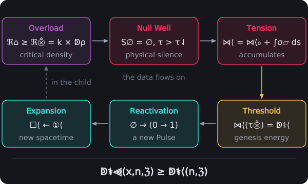
The Universal Genesis Process. A Null Well forms where local recursion reaches the critical density, ℜ⌂ ≥ ℜ⨶ = k × ↁρ, and falls physically silent while its data flows on. Tension accumulates until the Data Energy reaches the genesis threshold, ↁ⚕⫷ ≥ ↁ⚕⟨; the Pulse restarts, ∅ → (0 → 1), and a new spacetime domain expands.
UniSphereal Consistency in Emergent Universes
The birth of a new universe does not simply replicate its parent; it emerges with modified parameters determined by the substrate lattice from which it is born. Binary Pulse Theory formalizes this through Parameter Scaling (G), where Planck time, the speed of light, gravitational constant, and Planck’s constant shift according to dimensionless scaling factors. These parameters cannot vary arbitrarily — their interdependence is constrained by strict dimensional consistency, ensuring that emergent universes occupy only stable regions of the multiverse landscape.
Emergent Universe parameters differ from parent Universe through substrate lattice modifications.
UniSphereal Universe Consistency Equations G
The UniSphereal Universe Consistency Equations define how fundamental constants rescale in emergent universes. Pulse time, light speed, and coupling constants shift with substrate scaling, but their ratios are bound by the dimensional constraint (α²·β⁵ = γ·δ), ensuring only stable universes persist.
UniSpheral Scaled Pulse Tempo (G)
⧗'(n,ℨ) = α(n,ℨ)·⧗(ℨ)
Dimensional analysis:
[𝕋]([∅], [ℨ]) = [𝕋]
[∅]([∅], [ℨ]) × [𝕋]([ℨ]) = [∅] × [𝕋]([ℨ]) = [∅] × [𝕋] = [𝕋]
[𝕋] = [𝕋] ✓ Valid PulseCore Verified ✓
Harmonic level scaling of fundamental pulse temporal duration
UniSpheral Modified Light Speed G
𝒞→'(n,ℨ) = β(n,ℨ)·𝒞→(ℨ)
Dimensional analysis:
[𝕃·𝕋⁻¹]([∅], [ℨ]) = [𝕃·𝕋⁻¹]
[∅]([∅], [ℨ]) × [𝕃·𝕋⁻¹] = [∅] × [𝕃·𝕋⁻¹] = [𝕃·𝕋⁻¹]
[𝕃·𝕋⁻¹] = [𝕃·𝕋⁻¹] ✓ Valid PulseCore Verified ✓
Harmonic level scaling of light speed with Zinf scaling
UniSpheral Altered Constants G
𝒢'(n,ℨ) = γ(n,ℨ)·𝒢(ℨ)
Dimensional analysis:
[𝕄⁻¹·𝕃³·𝕋⁻²]([∅], [ℨ]) = [𝕄⁻¹·𝕃³·𝕋⁻²]
[∅]([∅], [ℨ]) × [𝕄⁻¹·𝕃³·𝕋⁻²]([ℨ]) = [∅] × [𝕄⁻¹·𝕃³·𝕋⁻²]([ℨ]) = [∅] × [𝕄⁻¹·𝕃³·𝕋⁻²] = [𝕄⁻¹·𝕃³·𝕋⁻²]
[𝕄⁻¹·𝕃³·𝕋⁻²] = [𝕄⁻¹·𝕃³·𝕋⁻²] ✓ Valid PulseCore Verified ✓
ℏ'(n,ℨ) = δ(n,ℨ)·ℏ(ℨ)
Dimensional analysis:
[𝕄·𝕃²·𝕋⁻¹]([∅], [ℨ]) = [𝕄·𝕃²·𝕋⁻¹]
[∅]([∅], [ℨ]) × [𝕄·𝕃²·𝕋⁻¹] = [∅] × [𝕄·𝕃²·𝕋⁻¹] = [𝕄·𝕃²·𝕋⁻¹]
[𝕄·𝕃²·𝕋⁻¹] = [𝕄·𝕃²·𝕋⁻¹] ✓ Valid PulseCore Verified ✓
Harmonic level scaling of fundamental constants with Zinf scaling
UniSpheral Dimensional Consistency Constraint G
α(n,ℨ)²·β(n,ℨ)⁵ = γ(n,ℨ)·δ(n,ℨ)
Dimensional analysis:
[∅]([∅], [ℨ])² × [∅]([∅], [ℨ])⁵ = [∅]² × [∅]([∅], [ℨ])⁵ = [∅] × [∅]([∅], [ℨ])⁵ = [∅] × [∅]⁵ = [∅] × [∅] = [∅]
[∅]([∅], [ℨ]) × [∅]([∅], [ℨ]) = [∅] × [∅]([∅], [ℨ]) = [∅] × [∅] = [∅]
[∅] = [∅] ✓ Valid PulseCore Verified ✓
Harmonic level scaling factor relationship maintaining dimensional consistency
Where:
- ⧗' [𝕋] - scaled Pulse Tempo (Planck time) in emergent universe
- α [∅] - Planck time scaling parameter
- ⧗ [𝕋] - parent universe Pulse Tempo (Planck time)
- 𝒞→' [𝕃·𝕋⁻¹] - modified light speed in emergent universe
- β [∅] - light speed scaling parameter
- 𝒞→ [𝕃·𝕋⁻¹] - parent universe light speed
- 𝒢' [𝕄⁻¹·𝕃³·𝕋⁻²] - altered gravitational constant in emergent universe
- γ [∅] - gravitational constant scaling parameter
- 𝒢 [𝕄⁻¹·𝕃³·𝕋⁻²] - parent universe gravitational constant
- ℏ' [𝕄·𝕃²·𝕋⁻¹] - modified Planck constant in emergent universe
- δ [∅] - Planck constant scaling parameter
- ℏ [𝕄·𝕃²·𝕋⁻¹] - parent universe Planck constant
➢ Emergent Universe parameters differ from parent Universe through substrate lattice modifications where scaling parameters determine physical constants in new universes, generating discrete multiverse landscapes where Universes cluster around stable parameter combinations through dimensional consistency constraints.
Polchinski's string-theoretic brane scenarios (Polchinski, 1998) generate discrete multiverse landscapes where Universes cluster around stable parameter combinations.
The UniSphereal Universe Consistency Equations demonstrate that emergent universes are not chaotic offshoots but lawful domains defined by substrate scaling. Their constants shift in harmony, constrained by dimensional balance, producing a structured multiverse where stability is mathematically enforced. In this way, BPT reframes cosmic diversity as the natural outcome of recursive consistency, where every new universe inherits order through scale rather than randomness.
2.2 Testable Predictions
- Discrete gravitational wave frequencies at integer multiples of ν_P ≈ 1.855 × 10⁴³ Hz reflecting Planck Pulse quantization, detectable through next-generation gravitational wave observatories with frequency resolution better than 10⁻⁶.
- Information echo signatures in cosmic microwave background corresponding to I⊶ topological encoding from pre-collapse states, measurable through precision analysis of CMB anisotropies with sensitivity better than 10⁻⁷.
- Periodic black hole evaporation modulations with period ①⥂⧗⌂ reflecting underlying Pulse structure in Hawking radiation, verifiable through precision measurements of black hole thermodynamics with sensitivity ΔT/T ~ 10⁻⁶.
- Quantized angular momentum in rotating black holes as J = n·ℏ with discrete substrate constraints n ∈ ℕ, detectable through gravitational wave strain pattern analysis during black hole mergers.
- Constants fixed within our universe: each universe's constants are set at its birth by its level and its parent's singularity and differ between universes following α²·β⁵ = γ·δ, so precision spectroscopy of quasar absorption lines should find no variation across our universe, with Δα/α consistent with zero at better than 10⁻⁶; a confirmed variation within our universe would count against this account.
These predictions, if confirmed, would support the computational foundation of spacetime, showing that:
- Black holes are computational phenomena, not purely gravitational
- Universe genesis follows precise mathematical rules rather than random cosmic accidents
- Physical constants differ between universes according to computational heritage, while staying fixed within each
- Time itself has discrete, digital structure at fundamental scales