Chapter 2 · Section 3
Null Wells (Black Holes) and the Birth of New Universes
What transforms cosmic death into cosmic birth? When a star collapses beyond traditional physics limits, Binary Pulse Theory fundamentally reconceptualizes gravitational singularities as Computational Genesis Mechanisms, instead of infinite-density mathematical breakdowns, BPT reveals critical endpoints as Null Wells — localized computational domains where binary recursive Pulses collapse into apparently paused states, where physical evolution halts as seen from outside while the data carries its information content on toward Universe creation. Where the collapsing star itself comes from, and why only the heaviest stars end this way, is set out in Part 2.9.
Hawking and Penrose's singularity theorems (Hawking & Penrose, 1970)⁹ suggested breakdown in physical laws, but BPT offers a different interpretation. Building upon the Planck Pulse framework from Part 2.2, Null Wells represent localized physical silences within active substrate — distinct from global computational states. Once accumulated boundary tension exceeds reactivation thresholds, these null states become genesis points for new Universe creation with modified fundamental constants determined by collapse parameters.
Guth's inflationary paradigm (Guth, 1981) echoes such reactivations, where rapid metric expansion establishes initial causal horizons. Understanding how gravitational collapse transforms into cosmic creation requires examining mathematical mechanisms connecting recursive density thresholds to Universe genesis processes.
Null Well (Black Hole) Formation and Collapse Evolution
Null Wells form not as singular points of infinite density, but as computational structures born when recursive demand outpaces substrate capacity. By treating collapse as an information-theoretic overload rather than a geometric singularity, Binary Pulse Theory reframes gravitational collapse as the transition from active recursion to apparent suspension, where physical evolution stalls but the data flows on. The Formation Condition and Collapse Evolution Equation formalize this process, showing both the trigger point for Null Well creation and the dynamic balance that governs how collapse unfolds.
Extending critical recursive density concepts from Part 2.2, Null Well formation occurs when local computational complexity exceeds substrate processing capacity.
Null Well Formation Condition G
ℜ⌂(x,τ,ℨ) ≥ ℜ⨶(ℨ) = k(ℨ) × ℏ(ℨ) × ↁρ(ℨ)
Dimensional analysis:
Where (from the book): ℜ⌂(x,τ,ℨ) [𝕄·𝕃⁻¹·𝕋⁻²], ℜ⨶(ℨ) [𝕄·𝕃⁻¹·𝕋⁻²], k(ℨ) [∅], ↁρ(ℨ) [𝕃⁻³·𝕋⁻¹], x [𝕃], τ [𝕋], ℨ [ℨ]
[𝕄·𝕃⁻¹·𝕋⁻²] ≥ [𝕄·𝕃⁻¹·𝕋⁻²]
[∅] × [𝕄·𝕃²·𝕋⁻¹] × [𝕃⁻³·𝕋⁻¹] = [𝕄·𝕃²·𝕋⁻¹] × [𝕃⁻³·𝕋⁻¹] = [𝕄·𝕃⁻¹·𝕋⁻²]
[𝕄·𝕃⁻¹·𝕋⁻²] ≥ [𝕄·𝕃⁻¹·𝕋⁻²] = [𝕄·𝕃⁻¹·𝕋⁻²] ✓ Valid PulseCore Verified ✓
Local recursion threshold triggering null well formation with Zinf scaling
Where:
- ℜ⌂(x,τ,ℨ) [𝕄·𝕃⁻¹·𝕋⁻²] – Local Recursion at position x, time τ, with Zinf scaling; local recursive tension density, an energy density, at primordial frequency
- ℜ⨶(ℨ) [𝕄·𝕃⁻¹·𝕋⁻²] – Zinf-scaled Critical Recursion threshold; the recursive tension density at which a null well forms (Critical Recursive Density, Part 2.2)
- k(ℨ) [∅] – Zinf-scaled proportionality constant; scaling factor relating Data density to critical threshold with primordial scaling
- ℏ(ℨ) [𝕄·𝕃²·𝕋⁻¹] – quantum action at Zinf scale; turns the Data density into an energy density
- ↁρ(ℨ) [𝕃⁻³·𝕋⁻¹] – Zinf-scaled Data Density; Data bits processed per unit volume per unit time (Part 1.8)
- x [𝕃] – spatial position parameter; location coordinate within substrate
- τ [𝕋] – temporal parameter; time coordinate in computational substrate
- ℨ [ℨ] – Zinf Unit; primordial temporal atom determining scaling
- ≥ [∅] – greater than or equal operator; critical threshold condition
- ⌂ [∅] – local indicator; specific location/domain
- ⨶ [∅] – threshold indicator; critical boundary
- × [∅] – multiplication operator
➢ Null Well Formation Condition establishes that when local recursion intensity exceeds the Zinf-scaled critical threshold determined by Data density, null well formation occurs as a protective substrate mechanism, creating localized computational voids that prevent recursive overflow and maintain substrate stability through systematic reset processes at primordial frequency scaling.
Null Well Collapse Evolution G
Null well collapse proceeds through four coupled evolutionary phases that systematically nullify substrate regions. Temporal evolution drives recursive intensity decay, spatial evolution contracts domain boundaries, energy evolution dissipates Data Energy, and recursive decay exponentially reduces structural complexity. These interconnected processes maintain computational stability through controlled reset mechanisms at Zinf-scaled primordial frequency.
Temporal Evolution
dℜ(x,τ,ℨ)/dτ = -γ(ℨ)ℜ(x,τ,ℨ)
Recursive intensity decay rate over time
Spatial Evolution
d☐(x,τ,ℨ)/dτ = -κ(ℨ)∇²☐(x,τ,ℨ)
Dimensional analysis:
Where (from the book): e [∅]
Read dimensionally: (☐(x,τ,ℨ)/τ) = -κ(ℨ) × (☐(x,τ,ℨ)/x²)
([𝕃] ÷ [𝕋]) = [𝕃·𝕋⁻¹]
[𝕃²·𝕋⁻¹] × ([𝕃] ÷ [𝕃²]) = [𝕃²·𝕋⁻¹] × [𝕃⁻¹] = [𝕃·𝕋⁻¹]
[𝕃·𝕋⁻¹] = [𝕃·𝕋⁻¹] ✓ Valid PulseCore Verified ✓
Space domain boundary contraction dynamics
Energy Evolution
d(ↁ⚕)/dτ = -λ(ℨ)ↁ⚕(x,τ,ℨ)
Data Energy dissipation during collapse
Recursive Decay
ℜ(τ,ℨ) = ℜ₀(ℨ)e^(-μ(ℨ)τ)
Exponential recursive structure breakdown
Where:
- ℜ(x,τ,ℨ) [𝕄·𝕃⁻¹·𝕋⁻²] – Zinf-scaled Recursion at position x, time τ; recursive tension density, an energy density
- ☐(x,τ,ℨ) [𝕃] – Zinf-scaled Space domain boundary at position x, time τ
- ↁ⚕(x,τ,ℨ) [𝕄·𝕃²·𝕋⁻²] – Zinf-scaled Data Energy at position x, time τ
- γ(ℨ) [𝕋⁻¹] – Zinf-scaled temporal decay coefficient
- κ(ℨ) [𝕃²·𝕋⁻¹] – Zinf-scaled spatial contraction (diffusion) coefficient
- λ(ℨ) [𝕋⁻¹] – Zinf-scaled energy dissipation coefficient
- μ(ℨ) [𝕋⁻¹] – Zinf-scaled recursive decay rate
- ℜ₀(ℨ) [𝕄·𝕃⁻¹·𝕋⁻²] – initial recursive tension density with Zinf scaling
- ∇ [𝕃⁻¹] – spatial gradient operator
- e [∅] – exponential function base
➢ The complete null well collapse evolution demonstrates how recursive intensity, spatial boundaries, Data Energy, and recursive structure simultaneously decay through coupled differential equations, establishing the comprehensive mathematical framework for substrate nullification processes that maintain computational stability through systematic collapse dynamics at Zinf-scaled primordial frequency.
Together, the Null Well Formation Condition and Null Well Collapse Evolution Equation establish Null Wells as finite, computable entities rather than pathological infinities. Collapse begins when recursive density crosses a critical threshold, but its evolution is shaped by nonlinear compression balanced against diffusion of tension through the substrate. The result is not a breakdown of physics, but a lawful suspension of physical state updates, preserving total information while the data flows on and activity shifts to boundary encoding. In this way, BPT transforms gravitational collapse into a process of apparent physical suspension, embedding conservation and continuity where classical theory predicted singular failure.
Null Well Information Encoding and Universe Genesis
In Binary Pulse Theory, the collapse of a universe into a Null Well does not erase its informational content. Instead, boundary topology acts as a storage medium, encoding the parent universe’s heritage in surface tension fields. This encoding provides the initialization data for child universes, transforming collapse from an end-state into a mechanism of continuity. Where classical cosmology predicts loss, BPT establishes inheritance, aligning with Smolin’s view of cosmological natural selection in which only universes that preserve information propagate their structure forward.
Within Null Wells, information from the parent Universe becomes encoded in boundary topology, preserving computational heritage for child Universe initialization. Smolin's cosmological natural selection (Smolin, 1997) views this as cosmic natural selection, where Universes capable of surviving collapse pass on "genetic" information.
By examining the Boundary Information Integral we can understand how cosmic natural selection operates through boundary tension field encoding parent Universe information content via information crystallization mechanisms that preserve computational heritage for child Universe initialization.
Null Well Boundary Data Information G
Null well boundaries preserve essential Data Information through three mechanisms: density integration, tension ratio normalization, and pure information field integration. These boundaries maintain information conservation during collapse while enabling systematic substrate recovery through controlled information preservation at Zinf-scaled primordial frequency.
Data Information Density Integration
ↁℹ∂(V,ℨ) = ∫_∂V ↁℹρ(x,ℨ) dA
Data Information density accumulated across boundary surface
Dimensionless Tension Ratio
ↁℹ∂(V,ℨ) = ∫_∂V (⋈(x,ℨ)/⋈₀(ℨ)) dA
Normalized tension field information content
Pure Data Information Field
ↁℹ∂(V,ℨ) = ∫_∂V ℹ(x,ℨ) dA
Direct information field integration
Where:
- ↁℹ∂(V,ℨ) [∅] – Zinf-scaled Data Information at boundary; computational information content across null well boundary surface
- ∫_∂V [∅] – surface integral over boundary ∂V; mathematical integration across null well boundary
- ↁℹρ(x,ℨ) [𝕃⁻²] – Zinf-scaled Data Information density at position x; information concentration per unit area with primordial scaling
- ⋈(x,ℨ) [𝕄·𝕃⁻¹·𝕋⁻²] – Zinf-scaled Tension at position x; stress field at boundary location with primordial scaling
- ⋈₀(ℨ) [𝕄·𝕃⁻¹·𝕋⁻²] – Zinf-scaled reference tension; normalization constant for dimensionless ratio
- ℹ(x,ℨ) [𝕃⁻²] – Zinf-scaled Information field at position x; pure dimensionless information content per unit area
- dA [𝕃²] – differential area element; infinitesimal surface area
- V [𝕃³] – null well volume; three-dimensional collapsed region
- ∂ [∅] – boundary operator; surface boundary indicator
- x [𝕃] – spatial position parameter; location coordinate on boundary surface
- ℨ [ℨ] – Zinf Unit; primordial temporal atom determining scaling
➢ The three formulations of Null Well Boundary Information Integration demonstrate complementary approaches to measuring Data Information content: density integration captures distributed information concentration, tension ratio normalization provides stress-based data information metrics, and pure information field integration measures direct computational data information flow, establishing comprehensive mathematical tools for analyzing information conservation and transformation across null well boundaries in computational substrate architecture.
Null Well Progeny Count Law G
N(L) = ℜ_U(L) / ↁℹ∂(V,ℨ) = 2^(L/3)
Dimensional analysis:
Where (from the book): ℜ_U(L) [∅], L [∅], 2^(L/3) [∅]
[∅]
[∅] ÷ [∅] = [∅]
[∅]
[∅] = [∅] = [∅] ✓ Valid PulseCore Verified ✓
Children a level-L universe seeds over its life: capacity divided by boundary information per well
Where:
- N(L) [∅] – number of child universes a universe at level L seeds; the number of its null wells that rupture
- ℜ_U(L) [∅] – UniSphere capacity at level L, 2^L (Two-Sided Growth, Chapter 1 Part D)
- ↁℹ∂(V,ℨ) [∅] – boundary information per null well, the surface integral above; an area law, so it scales as ℜ_U^(2/3)
- L [∅] – the universe's level
- 2^(L/3) [∅] – the remaining spatial third: capacity is a three-bit volume count, boundary cost is its two-thirds power
Level | Children |
|---|---|
0 (the Zinf universe) | 1 |
1, 2 | 1 |
3 | 2 |
6 | 4 |
201 (our parent's level: our siblings) | 1.5 × 10²⁰ |
202 (our universe) | 2^(202/3) ≈ 1.86 × 10²⁰ |
➢ The boundary integral carries the information a child inherits, and it is a surface integral: the cost of a child goes as the well's area, the holographic form of the Bekenstein bound in Chapter 1 Part D. The count is what remains, one spatial third of the capacity. The law seeds the Zinf universe exactly one child, the first rupture, and does not reach two children until level 3. For our universe it gives 1.86 × 10²⁰ children: the null wells that rupture, which are the black holes above the Standard Genesis mass ratio in the classification of Part 2.8. The observed count of stellar-mass black holes is 2 × 10¹⁹ to 10²⁰. Spin lowers the area of a well, by half at maximal spin, and so raises the count by at most a factor of two and brings the rupture sooner; high-spin lineages seed more, sooner, and pass the trait on through ⟪C⟫, which is the cosmological natural selection of Smolin and the reason our own origin is a near-maximal Kerr–Kerr merger. Because every level's children seed more than their parents did, the population at level L is ∏ 2^(k/3) over k < L: at our level about 2⁶⁷⁶⁷ ≈ 10²⁰³⁷ universes, with the last level dominating the whole UniSphere census.
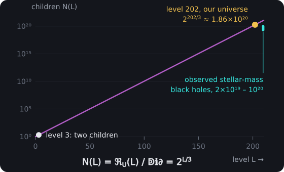
The Null Well Progeny Count Law. A universe at level L seeds N(L) = ℜ_U(L) / ↁℹ∂ = 2^(L/3) children: one at level 0, two at level 3, and 2^(202/3) ≈ 1.86 × 10²⁰ at our level, against an observed 2 × 10¹⁹ to 10²⁰ stellar-mass black holes.
The Boundary Information Integral establishes how cosmic natural selection functions through boundary tension field encoding parent Universe information content, demonstrating information crystallization mechanisms where boundary topology preserves computational heritage for child Universe initialization, enabling Universes capable of surviving collapse to pass genetic information through surface integration that encodes parent Universe characteristics within null well boundaries for subsequent cosmic rebirth and evolutionary continuity. The Boundary Information Integral formalizes this process, showing that surface tension fields integrate into dimensionless information content that can seed new universes.
Collapse thus becomes an act of encoding: information crystallizes at the boundary, is carried through the rupture, and reemerges at genesis. In this framework, cosmic evolution is not random variation but recursive inheritance, where universes capable of sustaining boundary encoding become progenitors in an ongoing lineage of cosmological rebirth.
Universe Genesis Mechanism and Reactivation
When a universe collapses into a Null Well, physical recursion appears to halt but information does not vanish. Instead, boundary topology becomes the archive of the parent domain, encoding its computational heritage into the surface of the Null Well. This mechanism ensures that child universes are not born from arbitrary initial conditions but from structured inheritance. In this way, BPT extends the logic of collapse and reactivation into a full cycle of cosmic continuity, showing how information transfer across boundaries provides the seed data for new universes.
A Null Well transitions to active genesis when accumulated boundary tension surpasses critical thresholds. By examining the Genesis Threshold Condition we can understand how active genesis operates through accumulated boundary tension surpassing critical thresholds determined by the Genesis Coupling Constant, the quantum action, the critical Data density and the Null Well Volume.
Genesis Threshold Condition G
⋈∂(V∅,ℨ) ≥ ⋈⟨(ℨ) =
k⟨(ℨ) · ℏ(ℨ) · ↁρ①(ℨ) · V∅(ℨ)
Dimensional analysis:
Where (from the book): ⋈∂(V∅,ℨ) [𝕄·𝕃²·𝕋⁻²], ⋈⟨(ℨ) [𝕄·𝕃²·𝕋⁻²], k⟨(ℨ) [∅], ↁρ①(ℨ) [𝕃⁻³·𝕋⁻¹], ⟨ [∅], ℨ [ℨ]
[𝕄·𝕃²·𝕋⁻²] ≥ [𝕄·𝕃²·𝕋⁻²]
[∅] × [𝕄·𝕃²·𝕋⁻¹] × [𝕃⁻³·𝕋⁻¹] × [𝕃³] = [𝕄·𝕃²·𝕋⁻¹] × [𝕃⁻³·𝕋⁻¹] × [𝕃³] = [𝕄·𝕃⁻¹·𝕋⁻²] × [𝕃³] = [𝕄·𝕃²·𝕋⁻²]
[𝕄·𝕃²·𝕋⁻²] ≥ [𝕄·𝕃²·𝕋⁻²] = [𝕄·𝕃²·𝕋⁻²] ✓ Valid PulseCore Verified ✓
Critical boundary tension threshold triggering universe genesis from null wells
Where:
- ⋈∂(V∅,ℨ) [𝕄·𝕃²·𝕋⁻²] – Zinf-scaled Boundary Tension accumulated across null well surface
- ⋈⟨(ℨ) [𝕄·𝕃²·𝕋⁻²] – Zinf-scaled Genesis Tension threshold
- k⟨(ℨ) [∅] – Zinf-scaled Genesis Coupling Constant
- ℏ(ℨ) [𝕄·𝕃²·𝕋⁻¹] – quantum action at Zinf scale; turns the Data density into an energy density, as E = ℏ × I × ω does for a count of bits (Part 3.1)
- ↁρ①(ℨ) [𝕃⁻³·𝕋⁻¹] – Zinf-scaled Pulse Density; the critical Data density, Data bits per unit volume per unit time (UniSpheral Data Density, Part 1.8)
- V∅(ℨ) [𝕃³] – Zinf-scaled Null Well Volume
- ∂ [∅] – boundary indicator
- ⟨ [∅] – genesis indicator
- ℨ [ℨ] – Zinf Unit
- ≥ [∅] – greater than or equal operator
➢ The Genesis Threshold Condition establishes that accumulated boundary tension must exceed the critical threshold determined by the Genesis Coupling Constant, the quantum action, the Zinf-scaled Pulse density and the Null Well volume (ℏ × ↁρ① is an energy per unit volume, so ℏ × ↁρ① × V∅ is an energy: [𝕄·𝕃²·𝕋⁻¹] × [𝕃⁻³·𝕋⁻¹] × [𝕃³] = [𝕄·𝕃²·𝕋⁻²]), triggering systematic universe genesis through computational substrate reactivation when sufficient stress energy accumulates at null well boundaries.
Genesis Process Phases:
- Tension Accumulation: T(τ) = T₀e^(λτ) through boundary stress concentration
- Critical Threshold: T(τ⨶) = T⇌ triggering reactivation
- Pulse Reactivation: 0 → 1 ascent initiating Prime Pulse bifurcation
- Spacetime Emergence: New metric g'_μν development through substrate geometry
- Recursive Expansion: Domain growth through Wavelength Scaling Law λ_n = λ₀ / n
The Boundary Information Integral reveals why reactivated universes differ yet remain coherent: parent information is crystallized into dimensionless form at the boundary, carried through the rupture, and released at rebirth. This transforms cosmological evolution into a recursive process where universes propagate their “genetic code” through collapse and reactivation. By embedding inheritance at the boundary, BPT frames the multiverse not as disconnected domains but as a lineage of universes, each shaped by the computational history of its predecessors.
UniSphereal Recursive Closure Framework
Having shown how universes collapse into Null Wells and reemerge through reactivation thresholds, we now identify the deeper rule that governs every recursion from the start: the UniSphereal Closure Framework. This law decides whether a process stabilizes into energy and structure or collapses into apparent silence, making it the universal checkpoint of existence.
The UniSphere does not permit recursion to run unchecked. Every process must resolve within a finite interval defined by the Zinf seed tick ℨ. The Closure Law establishes the fundamental boundary: if recursive completion occurs within one seed unit, the full Zinf cycle of two data rhythms ↁℨ⧖, stability is achieved and energy is generated; if not, collapse ensues and the recursion falls into a null well. This law is the gatekeeper of existence, deciding whether a pulse becomes structured or vanishes back into void.
UniSphereal Closure Law G
The UniSpheral Closure Law establishes the critical temporal boundary that determines whether computational processes maintain substrate stability or trigger protective collapse mechanisms. This law operates at the UniSphereal Pulse Period, creating the fundamental constraint that governs all recursive operations across the cosmic architecture through the complete computational cycle of the entire UniSphere.
UniSphereal Stability Condition G
τ⟫(ℨ) ≤ ☫⥂⁻¹
Dimensional analysis:
Where (from the book): τ⟫(ℨ) [⧖], ☫⥂⁻¹ [⧖], ℨ [ℨ]
[⧖] ≤ [⧖] ✓ Valid PulseCore Verified ✓
Critical closure time constraint for substrate computational stability
UniSphereal Collapse Condition G
τ⟫(ℨ) > ☫⥂⁻¹
Dimensional analysis:
Where (from the book): τ⟫(ℨ) [⧖], ☫⥂⁻¹ [⧖], ℨ [ℨ]
[⧖] > [⧖] ✓ Valid PulseCore Verified ✓
Critical closure time threshold triggering substrate collapse
Where:
- τ⟫(ℨ) [⧖] – Zinf-scaled closure time; duration required for computational process completion at primordial frequency
- ☫⥂⁻¹ [⧖] – UniSphereal Pulse Period; complete computational cycle duration of the entire UniSphere
- ☫⥂ [⧖⁻¹] – UniSphereal Pulse Rate; fundamental frequency of complete UniSphere computational cycles
- ☫ [∅] – UniSphereal indicator; entire computational universe architecture
- ℨ [ℨ] – Zinf Unit; primordial temporal atom
- ≤ [∅] – less than or equal operator; stability constraint condition
- > [∅] – greater than operator; collapse triggering condition
- ⟫ [∅] – closure indicator; completion/resolution process
- ⁻¹ [∅] – inverse operator; reciprocal mathematical function
➢ The UniSphereal Closure Law establishes that computational processes must complete within one complete UniSpheral Pulse Period to maintain substrate stability, while those exceeding this fundamental cycle duration trigger protective null well formation, creating the overarching temporal constraint that prevents recursive overflow by aligning all computational operations with the master rhythm of the entire cosmic architecture.
Recursive closure dynamics demonstrate how the UniSphere enforces stability through Zinfinity. If closure occurs within ℨ-based bounds, emergence succeeds, and energy manifests as real computation. If closure exceeds the limit, collapse follows, producing Null Wells. In this way, the constants of physics and the existence of matter itself are not arbitrary: they are direct consequences of Zinfinity’s ceiling and the recursive architecture of the UniSphere. Closure is thus the operational heartbeat of reality — the law that determines whether recursion produces structure or apparent silence.
The UniSphereal Closure Law thus unifies collapse, null wells, and reactivation under a single principle: recursion succeeds if it closes within the Zinf seed interval, or it fails, and its physical evolution appears to fall still while the data runs on through the rupture. It is the computational boundary condition that explains why universes can exist at all — and why collapse is as natural a law as emergence.
Universe Parameter Inheritance and UniSphere Structure
Universes that emerge from Null Wells do not begin with random constants; they inherit them through structured transformations governed by the UniSphere. The Explicit Scaling Functions define how collapse observables — density, boundary information, tension, and entropy — map directly into rescaled constants for the child universe. This framework shows how physics itself is passed down, transforming collapse from a destructive end into a generative act of inheritance.
By examining the Explicit Scaling Functions and Dimensional Consistency Constraint we can understand how finely tuned constants operate through parameter inheritance from computational collapse conditions using scaling functions that determine child Universe physics via collapse density, boundary information, tension, and entropy ratios, while discrete multiverse landscapes operate through parameter combinations clustering around stable configurations that ensure mathematical coherence across parameter inheritance from computational collapse conditions.
Universe-Specific Emergent Parameters G
Child Universes inherit modified constants determined by Null Well collapse parameters, transforming physics understanding from universal principles to Domain-Specific Emergent Properties.
UniSphereal Collapse Scaling Relations G
During null well collapse, fundamental physical constants undergo systematic modifications through dimensionless scaling functions. These relations demonstrate how Pulse tempo, light speed, gravitational constant, and Planck constant adapt to substrate collapse conditions based on collapse density, boundary information, boundary tension, and entropy changes while maintaining dimensional consistency through Zinf-scaled relationships.
Modified Pulse Tempo
⧗'(ℨ) = α(ↁρ⟫,ℨ) · ⧗(ℨ)
Dimensional analysis:
Where (from the book): ⧗'(ℨ) [𝕋], 𝒞→'(ℨ) [𝕃·𝕋⁻¹], 𝒢'(ℨ) [𝕄⁻¹·𝕃³·𝕋⁻²], ℏ'(ℨ) [𝕄·𝕃²·𝕋⁻¹], α(ↁρ⟫,ℨ) [∅], β(ↁℹ∂,ℨ) [∅], γ(⋈∂,ℨ) [∅], δ(S∅,ℨ) [∅], ⧗(ℨ) [𝕋], 𝒢(ℨ) [𝕄⁻¹·𝕃³·𝕋⁻²], ↁρ⟫ [𝕃⁻³·𝕋⁻¹], ↁℹ∂ [∅], ⋈∂ [∅], ℨ [ℨ]
[𝕋]
[∅] × [𝕋] = [𝕋]
[𝕋] = [𝕋] ✓ Valid PulseCore Verified ✓
Pulse temporal duration scaling with collapse density
Altered Light Speed
𝒞→'(ℨ) = β(ↁℹ∂,ℨ) · 𝒞→(ℨ)
Dimensional analysis:
Where (from the book): ⧗'(ℨ) [𝕋], 𝒞→'(ℨ) [𝕃·𝕋⁻¹], 𝒢'(ℨ) [𝕄⁻¹·𝕃³·𝕋⁻²], ℏ'(ℨ) [𝕄·𝕃²·𝕋⁻¹], α(ↁρ⟫,ℨ) [∅], β(ↁℹ∂,ℨ) [∅], γ(⋈∂,ℨ) [∅], δ(S∅,ℨ) [∅], ⧗(ℨ) [𝕋], 𝒢(ℨ) [𝕄⁻¹·𝕃³·𝕋⁻²], ↁρ⟫ [𝕃⁻³·𝕋⁻¹], ↁℹ∂ [∅], ⋈∂ [∅], ℨ [ℨ]
[𝕃·𝕋⁻¹]
[∅] × [𝕃·𝕋⁻¹] = [𝕃·𝕋⁻¹]
[𝕃·𝕋⁻¹] = [𝕃·𝕋⁻¹] ✓ Valid PulseCore Verified ✓
Data Information propagation rate modification with boundary information
Modified Gravitational Constant
𝒢'(ℨ) = γ(⋈∂,ℨ) · 𝒢(ℨ)
Dimensional analysis:
Where (from the book): ⧗'(ℨ) [𝕋], 𝒞→'(ℨ) [𝕃·𝕋⁻¹], 𝒢'(ℨ) [𝕄⁻¹·𝕃³·𝕋⁻²], ℏ'(ℨ) [𝕄·𝕃²·𝕋⁻¹], α(ↁρ⟫,ℨ) [∅], β(ↁℹ∂,ℨ) [∅], γ(⋈∂,ℨ) [∅], δ(S∅,ℨ) [∅], ⧗(ℨ) [𝕋], 𝒢(ℨ) [𝕄⁻¹·𝕃³·𝕋⁻²], ↁρ⟫ [𝕃⁻³·𝕋⁻¹], ↁℹ∂ [∅], ⋈∂ [∅], ℨ [ℨ]
[𝕄⁻¹·𝕃³·𝕋⁻²]
[∅] × [𝕄⁻¹·𝕃³·𝕋⁻²] = [𝕄⁻¹·𝕃³·𝕋⁻²]
[𝕄⁻¹·𝕃³·𝕋⁻²] = [𝕄⁻¹·𝕃³·𝕋⁻²] ✓ Valid PulseCore Verified ✓
Spacetime curvature parameter scaling with boundary tension
Scaled Planck Constant
ℏ'(ℨ) = δ(S∅,ℨ) · ℏ(ℨ)
Dimensional analysis:
Where (from the book): ⧗'(ℨ) [𝕋], 𝒞→'(ℨ) [𝕃·𝕋⁻¹], 𝒢'(ℨ) [𝕄⁻¹·𝕃³·𝕋⁻²], ℏ'(ℨ) [𝕄·𝕃²·𝕋⁻¹], α(ↁρ⟫,ℨ) [∅], β(ↁℹ∂,ℨ) [∅], γ(⋈∂,ℨ) [∅], δ(S∅,ℨ) [∅], ⧗(ℨ) [𝕋], 𝒢(ℨ) [𝕄⁻¹·𝕃³·𝕋⁻²], ↁρ⟫ [𝕃⁻³·𝕋⁻¹], ↁℹ∂ [∅], ⋈∂ [∅], ℨ [ℨ]
[𝕄·𝕃²·𝕋⁻¹]
[∅] × [𝕄·𝕃²·𝕋⁻¹] = [𝕄·𝕃²·𝕋⁻¹]
[𝕄·𝕃²·𝕋⁻¹] = [𝕄·𝕃²·𝕋⁻¹] ✓ Valid PulseCore Verified ✓
Quantum action unit modification with entropy changes
Where:
- ⧗'(ℨ) [𝕋] – Modified unified Pulse Tempo; altered fundamental temporal duration operating simultaneously across Data computational substrate and Physical manifestation layers
- 𝒞→'(ℨ) [𝕃·𝕋⁻¹] – Modified unified Light Speed; altered information propagation rate affecting both computational processes and physical phenomena
- 𝒢'(ℨ) [𝕄⁻¹·𝕃³·𝕋⁻²] – Modified unified Gravitational Constant; altered spacetime curvature parameter operating across Data-Physical architecture
- ℏ'(ℨ) [𝕄·𝕃²·𝕋⁻¹] – Modified unified Planck Constant; altered quantum action unit affecting both computational substrate and physical manifestation
- α(ↁρ⟫,ℨ) [∅] – Zinf-scaled collapse density scaling function; dimensionless modification based on Data collapse density
- β(ↁℹ∂,ℨ) [∅] – Zinf-scaled boundary information scaling function; dimensionless modification based on Data boundary information
- γ(⋈∂,ℨ) [∅] – Zinf-scaled boundary tension scaling function; dimensionless modification based on boundary tension
- δ(S∅,ℨ) [∅] – Zinf-scaled entropy scaling function; dimensionless modification based on entropy changes
- ⧗(ℨ) [𝕋] – base unified Pulse Tempo; fundamental temporal duration operating across Data-Physical architecture
- 𝒞→(ℨ) [𝕃·𝕋⁻¹] – base unified Light Speed; fundamental information propagation rate across computational and physical domains
- 𝒢(ℨ) [𝕄⁻¹·𝕃³·𝕋⁻²] – base unified Gravitational Constant; fundamental spacetime curvature parameter
- ℏ(ℨ) [𝕄·𝕃²·𝕋⁻¹] – base unified Planck Constant; fundamental quantum action unit
- ↁρ⟫ [𝕃⁻³·𝕋⁻¹] – Data collapse density parameter; computational density during null well formation
- ↁℹ∂ [∅] – Data boundary information parameter; information content at null well boundaries
- ⋈∂ [∅] – boundary tension parameter; stress accumulation at null well interfaces
- S∅ [∅] – entropy parameter; disorder measure during collapse processes
- ℨ [ℨ] – Zinf Unit; primordial temporal atom determining scaling
➢ The UniSphereal Collapse Scaling Relations demonstrate how Data substrate parameters drive coordinated modifications in unified constants that inherently operate across both computational and physical layers, establishing that fundamental constants are not separate entities requiring bridging but unified structures naturally spanning Data-Physical architecture, with collapse processes originating in computational substrate (ↁρ⟫, ↁℹ∂) directly altering the temporal, propagation, curvature, and quantum parameters governing both domains simultaneously.
UniSphereal Explicit Scaling Functions G
The UniSphereal Explicit Scaling Functions map collapse observables to dimensionless scaling factors. Each function links a Data substrate boundary variable — collapse density, boundary information, tension, or entropy — to the rescaling of unified constants. Together they define the transformation rules that govern how emergent universes inherit modified parameters from collapse conditions.
Collapse Density Scaling Function G
α(ↁρ⟫,ℨ) = (ↁρ①(ℨ)/ↁρ⟫(ℨ))^(1/2)
Dimensional analysis:
Where (from the book): α(ↁρ⟫,ℨ) [∅], ↁρ①(ℨ) [𝕃⁻³·𝕋⁻¹], ↁρ⟫(ℨ) [𝕃⁻³·𝕋⁻¹], β(ↁℹ⟫⟪,ℨ) [∅], ↁℹ⟫⟪(ℨ) [1ᵇ], ↁℹ⥂(ℨ) [1ᵇ], γ(⋈⟫⟪,ℨ) [∅], ⋈⟫⟪(ℨ) [𝕄·𝕃²·𝕋⁻²], ⋈⥂(ℨ) [𝕄·𝕃²·𝕋⁻²], δ(S∅,ℨ) [∅], S⥂(ℨ) [∅], S∅(ℨ) [∅], exp [∅], ℨ [ℨ]
[∅]
([𝕃⁻³·𝕋⁻¹] ÷ [𝕃⁻³·𝕋⁻¹])^([∅] ÷ [∅]) = ([𝕃⁻³·𝕋⁻¹] ÷ [𝕃⁻³·𝕋⁻¹])^([∅]) = [∅]^([∅]) = [∅]
[∅] = [∅] ✓ Valid PulseCore Verified ✓
Controls Pulse tempo rescaling through critical collapse density
Boundary Data Scaling Function G
β(ↁℹ⟫⟪,ℨ) = exp(-ↁℹ⟫⟪(ℨ)/ↁℹ⥂(ℨ))
Dimensional analysis:
[∅]([1ᵇ], [ℨ]) = [∅]
exp([1ᵇ]([ℨ]) ÷ [1ᵇ]([ℨ])) = exp([1ᵇ] ÷ [1ᵇ]([ℨ])) = exp([1ᵇ] ÷ [1ᵇ]) = exp([∅]) = [∅]
[∅] = [∅] ✓ Valid PulseCore Verified ✓
Controls light speed rescaling as information escapes boundary coupling interfaces
Boundary Tension Scaling Function G
γ(⋈⟫⟪,ℨ) = (⋈⟫⟪(ℨ)/⋈⥂(ℨ))^(1/3)
Dimensional analysis:
Where (from the book): α(ↁρ⟫,ℨ) [∅], ↁρ①(ℨ) [𝕃⁻³·𝕋⁻¹], ↁρ⟫(ℨ) [𝕃⁻³·𝕋⁻¹], β(ↁℹ⟫⟪,ℨ) [∅], ↁℹ⟫⟪(ℨ) [1ᵇ], ↁℹ⥂(ℨ) [1ᵇ], γ(⋈⟫⟪,ℨ) [∅], ⋈⟫⟪(ℨ) [𝕄·𝕃²·𝕋⁻²], ⋈⥂(ℨ) [𝕄·𝕃²·𝕋⁻²], δ(S∅,ℨ) [∅], S⥂(ℨ) [∅], S∅(ℨ) [∅], exp [∅], ℨ [ℨ]
[∅]
([𝕄·𝕃²·𝕋⁻²] ÷ [𝕄·𝕃²·𝕋⁻²])^([∅] ÷ [∅]) = ([𝕄·𝕃²·𝕋⁻²] ÷ [𝕄·𝕃²·𝕋⁻²])^([∅]) = [∅]^([∅]) = [∅]
[∅] = [∅] ✓ Valid PulseCore Verified ✓
Controls gravitational constant rescaling through boundary tension coupling
Entropy Scaling Function G
δ(S∅,ℨ) = (S⥂(ℨ)/S∅(ℨ))^(1/4)
Dimensional analysis:
Where (from the book): α(ↁρ⟫,ℨ) [∅], ↁρ①(ℨ) [𝕃⁻³·𝕋⁻¹], ↁρ⟫(ℨ) [𝕃⁻³·𝕋⁻¹], β(ↁℹ⟫⟪,ℨ) [∅], ↁℹ⟫⟪(ℨ) [1ᵇ], ↁℹ⥂(ℨ) [1ᵇ], γ(⋈⟫⟪,ℨ) [∅], ⋈⟫⟪(ℨ) [𝕄·𝕃²·𝕋⁻²], ⋈⥂(ℨ) [𝕄·𝕃²·𝕋⁻²], δ(S∅,ℨ) [∅], S⥂(ℨ) [∅], S∅(ℨ) [∅], exp [∅], ℨ [ℨ]
[∅]
([∅] ÷ [∅])^([∅] ÷ [∅]) = ([∅] ÷ [∅])^([∅]) = [∅]^([∅]) = [∅]
[∅] = [∅] ✓ Valid PulseCore Verified ✓
Controls quantum action rescaling based on entropy ratios
Where:
- α(ↁρ⟫,ℨ) [∅] – Collapse density scaling function; dimensionless Pulse Tempo modification based on Data density ratios
- ↁρ①(ℨ) [𝕃⁻³·𝕋⁻¹] – Critical Data density; threshold density for stable Pulse operations at Zinf scale
- ↁρ⟫(ℨ) [𝕃⁻³·𝕋⁻¹] – Data collapse density; actual computational density during null well formation
- β(ↁℹ⟫⟪,ℨ) [∅] – Boundary Data scaling function; dimensionless light speed modification based on coupling information ratios
- ↁℹ⟫⟪(ℨ) [1ᵇ] – Data interface coupling information; information content escaping boundary coupling interfaces
- ↁℹ⥂(ℨ) [1ᵇ] – Pulse Rate information; characteristic information content per complete binary cycle
- γ(⋈⟫⟪,ℨ) [∅] – Boundary tension scaling function; dimensionless gravitational modification based on coupling tension ratios
- ⋈⟫⟪(ℨ) [𝕄·𝕃²·𝕋⁻²] – Boundary coupling tension; stress accumulation during interface coupling processes
- ⋈⥂(ℨ) [𝕄·𝕃²·𝕋⁻²] – Pulse Rate tension; characteristic tension per complete binary cycle
- δ(S∅,ℨ) [∅] – Entropy scaling function; dimensionless quantum action modification based on entropy ratios
- S⥂(ℨ) [∅] – Pulse Rate entropy; characteristic entropy per complete binary cycle
- S∅(ℨ) [∅] – Collapse entropy; disorder measure during null well formation
- exp [∅] – Exponential function; natural exponential operation
- ℨ [ℨ] – Zinf Unit; primordial temporal atom
- ⟫⟪ [∅] – Interface coupling indicator; marks dynamic coupling/conversion processes
- ⟫ [∅] – Collapse indicator; marks parameters during null well formation
➢ The scaling functions establish how Data substrate collapse conditions determine unified constant inheritance through systematic ratios: density ratios control temporal scaling, interface coupling information governs propagation speed through exponential relationships, boundary tension coupling modifies spacetime curvature, and entropy ratios adjust quantum action parameters, demonstrating that universal constants inherit their values from computational collapse architecture through precise mathematical relationships operating across coupling interfaces where collapsed domains transition into emergent universes.
Dimensional Consistency Constraint G
α² · β⁵ = γ · δ
Where:
- α [∅] – Pulse Tempo scaling function; dimensionless modification for temporal duration
- β [∅] – light speed scaling function; dimensionless modification for information propagation rate
- γ [∅] – gravitational scaling function; dimensionless modification for spacetime curvature parameter
- δ [∅] – quantum action scaling function; dimensionless modification for unified action unit
Dimensional analysis:
Where (from the book): α [∅], β [∅], γ [∅], δ [∅]
[∅] × [∅] = [∅]
[∅] × [∅] = [∅]
[∅] = [∅] ✓ Valid PulseCore Verified ✓
➢ The dimensional consistency constraint ensures that all scaling functions maintain proper relationships during collapse processes, where the square of the Pulse Tempo scaling times the fifth power of the light speed scaling balances the product of gravitational and quantum action scaling, as the Planck time √(ℏ𝒢/𝒞→⁵) requires, preserving the fundamental dimensional structure that connects Pulse Tempo, information propagation, spacetime curvature, and quantum action across unified constant modifications during null well collapse and universe genesis.
The Dimensional Consistency Constraint generates discrete multiverse landscapes where parameter combinations cluster around stable configurations. Penrose's "cyclic Universe" concept (Penrose, 2010) shares similarities with new Universes branching from black holes.
Explicit Scaling Functions and the UniSphereal Dimensional Consistency Constraint show how finely tuned constants arise through parameter inheritance from computational collapse. Planck time scales with collapse density, light speed with exponential information decay, gravity with boundary tension, and Planck’s constant with entropy ratios. Bound by the consistency constraint, these functions generate a discretized multiverse where universes cluster around stable attractors rather than scattering into randomness. In this way, universes branching from black holes inherit Domain-Specific Emergent Properties, offering an account of both the fine-tuning of our constants and the recursive continuity of the UniSphere.
2.3 Testable Predictions
- Discrete gravitational wave frequencies: at integer multiples of ν_P ≈ 1.855 × 10⁴³ Hz reflecting Planck Pulse quantization, detectable through next-generation gravitational wave observatories with frequency resolution better than 10⁻⁶.
- Information echo signatures: in cosmic microwave background corresponding to I⊶ topological encoding from pre-collapse states, measurable through precision analysis of CMB anisotropies with sensitivity better than 10⁻⁷.
- Periodic black hole evaporation modulations: with period ①⥂⧗⌂ reflecting underlying Pulse structure in Hawking radiation, verifiable through precision measurements of black hole thermodynamics with sensitivity ΔT/T ~ 10⁻⁶.
- Quantized angular momentum: in rotating black holes as J = n·ℏ with discrete substrate constraints n ∈ ℕ, detectable through gravitational wave strain pattern analysis during black hole mergers.
- Constants fixed within our universe: constants differ between universes following α²·β⁵ = γ·δ but are fixed within each, so precision spectroscopy of quasar absorption lines should find Δα/α consistent with zero at better than 10⁻⁶; a confirmed variation within our universe would count against this account.
These predictions, if confirmed, would indicate that Universe genesis follows computational rules, showing that:
- Multiple Universes exist with systematically varying physical constants
- Cosmic evolution follows computational inheritance patterns
- Black hole formation creates rather than destroys information
- Reality consists of interconnected computational domains with shared heritage