Chapter 5 · Section 2
Quantum Phenomena as Computational Emergence
BPT proposes that wave functions and probabilities emerge naturally from binary computation, and approaches the measurement problem that has puzzled physicists for a century as computational forcing by the environment. The discrete, deterministic operations of binary substrate give rise to quantum mechanics through finite-resolution recursive Pulse dynamics, attributing probabilistic behavior not to intrinsic randomness but to emergent consequences of Phase Ambiguity in recursive systems. These phase states are not local hidden variables carried across space, so this determinism stands with Bell's theorem; Entanglement Through Shared Ancestry, below, shows how.
Hardy's axiomatic reformulation of quantum theory (Hardy, 2005)⁸ emphasized need for fundamental principles underlying quantum behavior. BPT replaces these axioms with substrate-level recursion constraints, reading quantum indeterminacy as a natural consequence of computational phase ambiguity rather than a fundamental postulate. Quantum Entanglement (G) emerges from shared Recursive Coherence (G) rather than nonlocal action, while Wave-Particle Duality (G) represents coherent versus localized Pulse configurations.
Feynman's recognition that physical behavior can be modeled through algorithmic evolution (Feynman, 1982)⁹ finds expression in BPT's substrate framework. Quantum mechanics becomes a special case of computable processes operating within finite recursive depth constraints.
Quantum Indeterminacy from Phase Ambiguity
Discovery: Quantum Indeterminacy emerges from local zones of unresolved Pulse phase within Recursive Substrate (G). When Recursive Depth R_d [∅] is insufficient to stabilize binary state transitions, the system exhibits Temporal Phase Ambiguity. By analyzing quantum indeterminacy from phase ambiguity we can understand how Quantum Indeterminacy emerges from local zones of unresolved Pulse phase within Recursive Substrate when Recursive Depth is insufficient to stabilize binary state transitions, while stochastic measurement outcomes emerge when observer interactions reveal unresolved phase states through quantum superposition representing computational processing states rather than mystical uncertainty, creating Temporal Phase Ambiguity that manifests as probabilistic behavior.
Quantum Transition Probability Equation
P(0→1) = 1/2 + δ × sin(ω×t + φ) [∅]
Where:
- P(0→1) is transition probability from state 0 to 1 [∅]
- δ is Phase Uncertainty Amplitude [∅]
- ω is substrate oscillation frequency [𝕋⁻¹]
- t is time [𝕋]
- φ is local phase offset [radians]
➢ Probabilistic behavior emerges from computational phase ambiguity rather than fundamental randomness — the Universe computes probabilities, not randomness through phase uncertainty amplitude and substrate oscillation frequency.
The Phase Uncertainty Amplitude δ measures computational ambiguity, while ω represents substrate oscillation frequency with ①⥂⧗⌂ = 2 × ①⥂⧖⌂ periodicity. Local phase offset φ emerges from Recursive State Evolution: S(n+1) = F[S(n), H(n), ℜₙ].
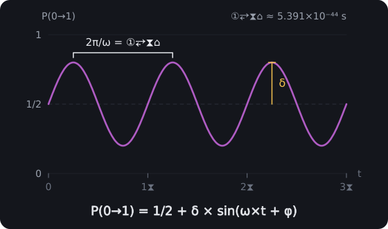
Transition Probability from Phase Ambiguity. P(0→1) = 1/2 + δ × sin(ω×t + φ) oscillates about 1/2 with the Phase Uncertainty Amplitude δ, repeating once every Pulse Tempo, 2π/ω = ①⥂⧗⌂ ≈ 5.391 × 10⁻⁴⁴ s. Shown with φ = 0; δ is not fixed by the theory.
Phase ambiguity manifests as stochastic measurement outcomes when observer interactions reveal unresolved phase states:
Quantum Superposition State Equation
|ψ⟩ = α|0⟩ + β|1⟩ where |α|² + |β|² = 1 [∅]
Where:
- |ψ⟩ is quantum state vector [∅]
- α, β are probability amplitudes [∅]
- |0⟩, |1⟩ are basis states [∅]
- |α|², |β|² are probability magnitudes [∅]
➢ Quantum superposition as representation of unresolved computational phase — not mystical uncertainty but computational processing states where probability amplitudes represent Recursive Amplitude Distributions rather than fundamental probabilistic weights.
In BPT, coefficients α, β represent Recursive Amplitude Distributions (G) rather than fundamental probabilistic weights. Aspect and colleagues' time-varying analyzer tests (Aspect et al., 1982) provide laboratory analogues for computationally bound entanglement correlations.
The quantum transition probability equation reveals how probabilistic behavior emerges from computational phase ambiguity while the quantum superposition state equation shows quantum states represent unresolved computational phase through Recursive Amplitude Distributions, where Phase Uncertainty Amplitude and substrate oscillation frequency create quantum indeterminacy through systematic phase uncertainty mechanisms, demonstrating superposition reflects computational processing states rather than fundamental uncertainty while maintaining normalization constraints ensuring probability conservation during measurement interactions governing binary state transition probabilities in recursive substrate architecture.
Measurement and Phase Resolution
Measurement collapse occurs when environmental recursion forces phase resolution. By examining measurement and phase resolution we can understand how measurement collapse occurs when environmental recursion forces phase resolution through Environmental Recursive Density exceeding critical thresholds for phase stabilization.
Phase Resolution Threshold Condition
R_d◌ > R_d⨶ [∅]
Where:
- R_d◌ is Environmental Recursive Density [∅]
- R_d⨶ is critical threshold for phase stabilization [∅]
Dimensional analysis:
Where (from the book): R_d◌ [∅], R_d⨶ [∅]
[∅] > [∅] ✓ Valid PulseCore Verified ✓
➢ Measurement as computational forcing rather than mysterious wavefunction collapse — the environment computes the answer through Environmental Recursive Density exceeding critical threshold to trigger phase stabilization.
Environmental Recursive Density (G) exceeding critical threshold triggers phase stabilization through Collapse Threshold Equation. Measurement represents computational forcing rather than mysterious wavefunction collapse.
The phase resolution threshold condition establishes how measurement represents computational forcing rather than mysterious wavefunction collapse, where Environmental Recursive Density exceeding critical threshold triggers phase stabilization through systematic environmental computation that resolves quantum phase ambiguity by forcing binary state transitions when recursive density surpasses stabilization requirements.
Entanglement Through Shared Ancestry
Quantum Entanglement (G) emerges from particles linked by common Prime Pulse Bifurcation origins. When particles form within the same discrete Pulse event, they maintain persistent recursive coherence through shared computational ancestry — offering a computational account of "spooky action at a distance."
By analyzing entanglement through shared ancestry, Bell parameter bounds, and Bell inequality test we can understand how Quantum Entanglement emerges from particles linked by common Prime Pulse Bifurcation origins that maintain persistent recursive coherence, while Bell inequality violations demonstrate that computational entanglement through non-separable recursive structures enables quantum correlations to exceed classical limits through correlation measurements revealing computational substrate effects that emerge from shared ancestry rather than fundamental nonlocality.
Recursive Correlation Function G
C(A,B) = ⟨Ψ_A(t) × Ψ_B(t)⟩_R [∅]
Where:
- C(A,B) is correlation function between particles A and B [∅]
- Ψ_A(t) is recursive state vector for particle A [∅]
- Ψ_B(t) is recursive state vector for particle B [∅]
- ⟨⟩_R denotes averaging over recursive substrate configurations [∅]
- A, B are particle identifiers [∅]
- t is time [𝕋]
➢ Entanglement through shared computational ancestry rather than nonlocal action — particles remember their computational family through persistent recursive coherence maintained from common Prime Pulse Bifurcation origins.
Substrate-Pulse Coupling: Ψ = P⬓ maintains correlation across arbitrary separations through computational memory.
Structural recursion naturally reproduces Bell inequality violations:
Bell Parameter Bounds
S● ≤ 2, S⊡ = 2√2 ≈ 2.83 [∅]
Where:
- S is Bell parameter [∅]
- S● is classical correlation bound ≤ 2 [∅]
- S⊡ is quantum correlation maximum = 2√2 ≈ 2.83 [∅]
- 2 is classical limit [∅]
- √2 is square root of 2 ≈ 1.414 [∅]
➢ Bell inequality violations emerge from non-separable recursive structures — computational entanglement exceeds classical limits through quantum correlation maximum surpassing classical bounds.
Bell Inequality Test
S = |E(a,b) - E(a,b') + E(a',b) + E(a',b')| [∅]
Where:
- S is Bell parameter from inequality test [∅]
- E(x,y) are correlation expectation values = ⟨cos(θ_x - θ_y)⟩_R [∅]
- a, b, a', b' are measurement setting parameters [∅]
- θ_x, θ_y are measurement angles [radians]
- ⟨⟩_R denotes averaging over recursive substrate configurations [∅]
➢ Correlation measurements in entangled systems revealing computational substrate effects where violation emerges from non-separable recursive structures rather than fundamental nonlocality, consistent with experimental observations.
Violation emerges from non-separable recursive structures rather than fundamental nonlocality, consistent with experimental observations by Aspect et al. (Aspect et al., 1982). This is how BPT meets Bell's theorem (Bell, 1964) and the loophole-free tests that confirm its violation (Hensen et al., 2015; Giustina et al., 2015; Shalm et al., 2015): no local hidden variables cross space; the correlation comes from the shared loop that all data passes through, the UniSphere and the Zinf; and no message can be sent faster than light, since each observer's result looks random until the results are compared by ordinary means.
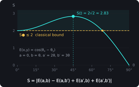
The Bell Parameter. With E(x,y) = cos(θ_x − θ_y) and settings a = 0, b = θ, a′ = 2θ, b′ = 3θ, the Bell parameter is S(θ) = |3 cos θ − cos 3θ|. It exceeds the classical bound S● ≤ 2 for 0° < θ < 68.5° and peaks at S⊡ = 2√2 ≈ 2.83 at θ = 45°.
The recursive correlation function reveals how entanglement operates through shared computational ancestry rather than nonlocal action while Bell parameter bounds show computational entanglement exceeds classical limits through non-separable recursive structures, and the Bell inequality test establishes how correlation expectation values create measurements exceeding classical bounds, demonstrating that quantum entanglement reflects computational family relationships where shared ancestry creates correlation strength impossible under classical physics through recursive substrate configurations that govern entangled system correlations via computational mechanisms rather than mysterious nonlocal action, maintaining consistency with experimental observations of Bell inequality violations.
Decoherence as Phase Resolution
Decoherence (G) results from Pulse collapse driven by increased Environmental Recursive Density (G). As quantum systems interact with environments possessing higher recursion complexity, indeterminate phase states transition into stable binary outputs.
By studying decoherence rate and time scale we can understand how quantum coherence degradation depends on the temperature and density ratios between environment and substrate through environmental coupling, following the decoherence rate of Part 7.3, Γ≋⦰ = γ◌ (T◌/T▱)² (ρ◌/ρ▱) [𝕋⁻¹], while the characteristic time for quantum coherence loss is the inverse of that rate.
Where:
- Γ≋⦰ is decoherence rate [𝕋⁻¹]
- γ◌ is environmental coupling [𝕋⁻¹]
- T◌ is environmental temperature [Θ]
- T▱ is substrate temperature [Θ]
- ρ◌ is environmental density [𝕄·𝕃⁻³]
- ρ▱ is substrate density [𝕄·𝕃⁻³]
In this law T▱ is chapter 7’s substrate temperature [Θ], not the substrate period T▱ of Part 5.3.
Dimensional analysis: [𝕋⁻¹] = [𝕋⁻¹] × ([Θ] ÷ [Θ])² × ([𝕄·𝕃⁻³] ÷ [𝕄·𝕃⁻³]) = [𝕋⁻¹] × [∅] × [∅] = [𝕋⁻¹] ✓ The decoherence rate equation is dimensionally consistent with expected rate units.
➢ Decoherence rate grows with the square of the environment-to-substrate temperature ratio and linearly with the density ratio — environment overpowers quantum computation through coupling that scales with environmental dominance and thermal activation.
Decoherence Time Scale
τ≋⦰ = 1/Γ≋⦰ [𝕋]
Where:
- τ≋⦰ is decoherence timescale [𝕋]
- Γ≋⦰ is decoherence rate (Part 7.3) [𝕋⁻¹]
Dimensional analysis:
Where (from the book): τ≋⦰ [𝕋]
[𝕋]
[∅] ÷ [𝕋⁻¹] = [𝕋]
[𝕋] = [𝕋] ✓ Valid PulseCore Verified ✓
➢ Characteristic time for quantum coherence loss: the inverse of the decoherence rate, so the hotter and denser the environment relative to the substrate, the sooner coherence is lost, following Zurek's decoherence formalism.
Environmental forcing matches Zurek's decoherence formalism (Zurek, 2003), though here collapse triggers from recursion density ratios rather than purely statistical state reduction.
The decoherence time scale equation establishes how quantum coherence loss occurs through environmental computational interference on timescales set by the inverse of the decoherence rate while the decoherence rate reveals how environmental density and temperature overpower system coherence through environmental coupling scaling quadratically with the temperature ratio and linearly with the density ratio, demonstrating that collapse triggers from recursion density ratios rather than statistical reduction when environmental computational capacity exceeds system capacity through precise mathematical relationships governing quantum-to-classical transitions via recursive substrate interactions while maintaining consistency with Zurek's decoherence formalism.
Physical Constants as Recursive Invariants
Physical constants emerge as constraints imposed by substrate architecture. Planck time ①⥂⧗⌂ ≈ 5.39 × 10^-44 seconds represents fundamental Pulse Tempo with ①⥂⧖⌂ = ①⥂⧗⌂/2. Speed of light follows 𝒞→ = l_p/①⥂⧗⌂ [𝕃·𝕋⁻¹] where l_p represents substrate lattice spacing, while Planck's constant becomes ℏ = E_p × ①⥂⧗⌂ [𝕄·𝕃²·𝕋⁻¹] with E_p as elementary Pulse energy.
By examining the fine structure constant we can understand how fundamental physical constants emerge from substrate recursive relationships, revealing the Universe's computational parameters through the ratio of recursive interaction strengths.
Fine Structure Constant
α = e²/(4π×ε_0×ℏ×c) ≈ 1/137 = R⧱⥣/R⧱⥥ [∅]
Where:
- α is fine structure constant ≈ 1/137 [∅]
- e is elementary charge [A T]
- ε_0 is vacuum permittivity [A² T⁴ M⁻¹ L⁻³]
- ℏ is reduced Planck constant [𝕄·𝕃²·𝕋⁻¹]
- c is speed of light [𝕃·𝕋⁻¹]
- R⧱⥣ is strong recursive interaction strength [∅]
- R⧱⥥ is weak recursive interaction strength [∅]
➢ Fundamental constant ratios emerge from substrate recursive relationships — the Universe's computational parameters where strong and weak recursive interaction strengths determine electromagnetic coupling through precise substrate architecture.
The fine structure constant equation establishes how electromagnetic coupling emerges from substrate recursive relationships where the ratio of strong to weak recursive interaction strengths determines fundamental physical constants, demonstrating that the Universe's computational parameters arise from precise recursive architecture governing electromagnetic interactions through substrate-mediated coupling mechanisms that produce the observed fine structure constant value.
Wave-Particle Duality and Coherence Regimes
Wave-like behavior corresponds to extended recursive coherence. By analyzing the wave function coherence equation and particle function localization equation we can understand how wave-like behavior corresponds to extended recursive coherence through distributed computational processing modulated by the Recursive Coherence Envelope, while particle-like behavior emerges from localized Pulse collapse through concentrated computational processing where Dirac delta function localization combines with squared coherence envelope magnitude.
Wave Function Coherence Equation
ψ∿(x,t) = A × exp(i×k×x - i×ω×t) × R(x,t) [𝕃⁻³/²]
Where:
- ψ∿(x,t) is wave function in coherence regime [𝕃⁻³/²]
- A is amplitude normalization [𝕃⁻³/²]
- k is wavenumber [𝕃⁻¹]
- ω is frequency [𝕋⁻¹]
- x is spatial position [𝕃]
- t is time [𝕋]
- R(x,t) is Recursive Coherence Envelope [∅]
- i is imaginary unit [∅]
Dimensional analysis:
Where (from the book): ψ∿(x,t) [𝕃⁻³/²], A [𝕃⁻³/²], k [𝕃⁻¹], ω [𝕋⁻¹], x [𝕃], t [𝕋], i [∅]
[𝕃⁻³/²]
[𝕃⁻³/²] × exp([∅] × [𝕃⁻¹] × [𝕃] - [∅] × [𝕋⁻¹] × [𝕋]) × [∅] = [𝕃⁻³/²] × exp([𝕃⁻¹] × [𝕃] - [∅] × [𝕋⁻¹] × [𝕋]) × [∅] = [𝕃⁻³/²] × exp([∅] - [∅] × [𝕋⁻¹] × [𝕋]) × [∅] = [𝕃⁻³/²] × exp([∅] - [𝕋⁻¹] × [𝕋]) × [∅] = [𝕃⁻³/²] × exp([∅] - [∅]) × [∅] = [𝕃⁻³/²] × exp([∅]) × [∅] = [𝕃⁻³/²] × [∅] × [∅] = [𝕃⁻³/²] × [∅] = [𝕃⁻³/²]
[𝕃⁻³/²] = [𝕃⁻³/²] ✓ Valid PulseCore Verified ✓
➢ Wave behavior through extended recursive coherence — distributed computational processing where Recursive Coherence Envelope modulates standard wave function to reflect substrate computational architecture.
Particle-like behavior emerges from localized Pulse collapse.
Particle Function Localization Equation
ψ⚛(x,t) = δ(x - x_0) × |R(x_0,t)|² [𝕃⁻³]
Where:
- ψ⚛(x,t) is wave function in particle regime [𝕃⁻³]
- δ(x - x_0) is Dirac delta function [𝕃⁻³]
- x is spatial position [𝕃]
- x_0 is localized position [𝕃]
- R(x_0,t) is Recursive Coherence Envelope at localized position [∅]
- |R(x_0,t)|² is squared magnitude of coherence envelope [∅]
- t is time [𝕋]
➢ Particle behavior through localized recursive collapse — concentrated computational processing where regime transitions depend on measurement interaction strength with Wave Regime when R⫤ << R▦ and Particle Regime when R⫤ >> R▦.
Regime transitions depend on measurement interaction strength, with Wave Regime when R⫤ << R▦ and Particle Regime when R⫤ >> R▦, where R⫤ is the measurement interaction strength and R▦ the system recursive density [∅].
The particle function localization equation establishes how particle behavior emerges through localized recursive collapse with Dirac delta function creating spatial localization and squared coherence envelope determining probability density, while the wave function coherence equation shows wave behavior emerges through extended recursive coherence combining amplitude normalization with phase factors, demonstrating that particle-like and wave-like behavior reflect concentrated versus distributed computational processing with regime transitions governed by measurement interaction strength relative to system coherence through mathematical relationships determining Wave versus Particle regime selection.
Uncertainty from Computational Limits
Heisenberg Uncertainty Principle (G) emerges from computational constraints rather than fundamental indeterminacy. By examining uncertainty from computational limits and recursive resolution uncertainty we can understand how the Heisenberg Uncertainty Principle emerges from computational constraints rather than fundamental indeterminacy through discrete substrate resolution limits, while fundamental computational resolution limits determine measurement precision through Minimum Recursive Resolution of the substrate governing uncertainty relationships in dimensionless recursive units.
Heisenberg Uncertainty Relation
Δx × Δp ≥ ℏ/2 = (E_p × ①⥂⧗⌂)/2 [𝕄·𝕃²·𝕋⁻¹]
Where:
- Δx is position uncertainty [𝕃]
- Δp is momentum uncertainty [𝕄·𝕃·𝕋⁻¹]
- ℏ is reduced Planck constant [𝕄·𝕃²·𝕋⁻¹]
- E_p is Planck energy [𝕄·𝕃²·𝕋⁻²]
- ①⥂⧗⌂ is Local Pulse Tempo (local Planck time) [𝕋]
Dimensional analysis:
Where (from the book): Δx [𝕃], Δp [𝕄·𝕃·𝕋⁻¹], ℏ [𝕄·𝕃²·𝕋⁻¹]
[𝕃] × [𝕄·𝕃·𝕋⁻¹] ≥ [𝕄·𝕃²·𝕋⁻¹] ÷ [∅] = [𝕄·𝕃²·𝕋⁻¹] ≥ [𝕄·𝕃²·𝕋⁻¹] ÷ [∅] = [𝕄·𝕃²·𝕋⁻¹] ≥ [𝕄·𝕃²·𝕋⁻¹]
([𝕄·𝕃²·𝕋⁻²] × [𝕋]) ÷ [∅] = [𝕄·𝕃²·𝕋⁻¹] ÷ [∅] = [𝕄·𝕃²·𝕋⁻¹]
[𝕄·𝕃²·𝕋⁻¹] ≥ [𝕄·𝕃²·𝕋⁻¹] = [𝕄·𝕃²·𝕋⁻¹] ✓ Valid PulseCore Verified ✓
➢ Uncertainty principle from discrete substrate resolution — computational precision limits, not mystical uncertainty where discrete substrate resolution creates fundamental measurement constraints.
Recursive Resolution Uncertainty
Δℜx × Δℜ⟡ ≥ R⥥/2 [∅]
Where:
- Δℜx is position uncertainty in recursive units [∅]
- Δℜ⟡ is momentum uncertainty in recursive units [∅]
- R⥥ is Minimum Recursive Resolution of substrate = ①⥂⧖⌂/①⥂⧗⌂ = 1/2 [∅]
- ①⥂⧖⌂ is Local Pulse Rhythm [𝕋]
- ①⥂⧗⌂ is Local Pulse Tempo (Planck time) [𝕋]
Dimensional analysis:
Where (from the book): Δℜx [∅], Δℜ⟡ [∅], R⥥ [∅]
[∅] × [∅] ≥ [∅] ÷ [∅] = [∅] ≥ [∅] ÷ [∅] = [∅] ≥ [∅] ✓ Valid PulseCore Verified ✓
➢ Fundamental computational resolution limit determining measurement precision where Minimum Recursive Resolution establishes substrate computational constraints governing uncertainty relationships.
The recursive resolution uncertainty and Heisenberg uncertainty relation establish how uncertainty emerges from computational constraints rather than fundamental indeterminacy, where discrete substrate resolution creates precision limits through Minimum Recursive Resolution and computational architecture constraints, demonstrating that position and momentum uncertainty products reflect substrate computational limits expressed through Planck-scale relationships and dimensionless recursive units governing measurement precision in discrete computational architecture.
Quantum Fields as Collective Dynamics
By analyzing quantum fields as collective dynamics and vacuum energy expectation we can understand how quantum fields emerge as collective excitations of computational substrate through coordinated binary processing via Pulse Creation/Annihilation Operators acting on substrate mode functions, while vacuum fluctuations emerge from substrate oscillations representing the Universe's background computation through Zero-point Recursive Oscillations.
Quantum Field Excitation Equation
φ(x,t) = Σ_k [a_k × u_k(x,t) + a_k† × u_k(x,t)] [various units]
Where:
- φ(x,t) is quantum field [various units]
- a_k are Pulse Creation/Annihilation Operators [∅]
- a_k† are Pulse Creation/Annihilation Operators (adjoint) [∅]
- u_k(x,t) are substrate mode functions [various units]
- k is mode index [∅]
- x is spatial position [𝕃]
- t is time [𝕋]
Dimensional analysis:
Where (from the book): φ(x,t) [various units], a_k [∅], a_k† [∅], u_k(x,t) [various units], k [∅], x [𝕃], t [𝕋]
Read dimensionally: φ(x,t) = (a_k × u_k(x,t) + a_k† × u_k(x,t))
[various units]
([∅] × [various units] + [∅] × [various units]) = ([various units] + [∅] × [various units]) = ([various units] + [various units]) = [various units]
[various units] = [various units] ✓ Valid PulseCore Verified ✓
➢ Quantum fields as collective excitations of computational substrate — coordinated binary processing through Pulse Creation/Annihilation Operators acting on substrate mode functions.
Zero-point Recursive Oscillations (G) provide computational origin for quantum field theory vacuum fluctuations.
Vacuum Energy Expectation Equation
⟨0|H|0⟩ = (1/2) × Σ_{k=1}^{∞} ℏ×ω_k [𝕄·𝕃²·𝕋⁻²]
Where:
- ⟨0|H|0⟩ is vacuum expectation value of Hamiltonian [𝕄·𝕃²·𝕋⁻²]
- ℏ is reduced Planck constant [𝕄·𝕃²·𝕋⁻¹]
- ω_k is frequency of mode k [𝕋⁻¹]
- k is mode index [∅]
Dimensional analysis:
Where (from the book): ⟨0|H|0⟩ [𝕄·𝕃²·𝕋⁻²], ℏ [𝕄·𝕃²·𝕋⁻¹], ω_k [𝕋⁻¹], k [∅]
Read dimensionally: ⟨0|H|0⟩ = (1/2) × ℏ×ω_k
[𝕄·𝕃²·𝕋⁻²]
([∅] ÷ [∅]) × [𝕄·𝕃²·𝕋⁻¹] × [𝕋⁻¹] = [∅] × [𝕄·𝕃²·𝕋⁻¹] × [𝕋⁻¹] = [𝕄·𝕃²·𝕋⁻¹] × [𝕋⁻¹] = [𝕄·𝕃²·𝕋⁻²]
[𝕄·𝕃²·𝕋⁻²] = [𝕄·𝕃²·𝕋⁻²] ✓ Valid PulseCore Verified ✓
➢ Vacuum fluctuations from substrate oscillations — the Universe's background computation where Zero-point Recursive Oscillations provide computational origin for quantum field theory vacuum fluctuations. Summed over every mode down to the Zinf, the sum gives about the Planck density, some 10¹²³ times the vacuum energy measured: the cosmological constant problem (Weinberg, 1989). The vacuum that gravitates is counted on its boundary instead, and Part 3.13 counts it so, as the Null Vacuum and its Vacuum Pressure.
The vacuum energy expectation equation establishes how vacuum fluctuations emerge from substrate oscillations through Zero-point Recursive Oscillations while the quantum field excitation equation shows how quantum fields emerge as collective excitations through Pulse Creation/Annihilation Operators acting on substrate mode functions, demonstrating that vacuum energy represents the Universe's background computation and quantum fields represent coordinated binary processing rather than fundamental entities while maintaining mathematical consistency with quantum field theory through precise operator algebra governing substrate mode excitations and requiring regularization to manage infinite summation over computational background activity.
5.2 Testable Predictions
- Discrete Energy Signatures: Ultra-high precision spectroscopy reveals temporal quantization effects with ①⥂⧖⌂ = ①⥂⧗⌂/2 periodicity, detectable in atomic transitions with frequency resolution better than 10^-18.
- Entanglement Modulations: Periodic fidelity variations in Bell experiments reflecting substrate oscillation frequencies at timescales around 10^-44 seconds.
- Computational Complexity Bounds: Quantum algorithm performance limited by substrate resolution constraints, observable in quantum computing systems with more than 1000 qubits.
- Phase Uncertainty Measurements: Environmental Recursive Density (G) variations detected through phase amplitude monitoring in isolated quantum systems.
These predictions would reframe quantum mechanics by showing that probabilistic behavior emerges from computational processes rather than fundamental randomness, establishing quantum theory as a special case of binary computation and opening pathways to engineering quantum effects through computational substrate manipulation.