Primordial Computational Foundation

Before the first Pulse, before time itself began, Binary Pulse Theory proposes the existence of Zero Substrate — fundamental computational foundation existing in temporal stasis. Unlike dynamic substrate explored in previous parts, Frame 0 (G) represents primordial boundary condition containing all structural information necessary for subsequent binary Pulse transitions while remaining temporally frozen with ∂S_0/∂t = 0.

This offers an account of the "something from nothing" problem through computational logic rather than metaphysical speculation. Causal set theory models spacetime as partially ordered sets without continuous background (Bombelli et al., 1987)²⁴, providing established approaches to pre-geometric reality paralleling BPT's Zero Substrate. In computational terms, Zero Substrate functions as halted universal quantum computer (Lloyd, 2006)⁶, its registers loaded with initial conditions but no clock cycle initiated.

The Pre-Geometric Phase (G) provides essential tension distributions, topological constraints, and information content driving all subsequent recursive evolution through Recursive State Evolution: S(n+1) = F[S(n), H(n), ℜₙ] once temporal dynamics activate.

Pre-Temporal Substrate Framework

Building upon Binary Substrate Reality (G) from Part 5.1, Zero Substrate consists of discrete spatial lattice D with position vectors x ∈ D arranged in quasi-crystalline structure supporting subsequent dimensional emergence. By examining the Zero Substrate Definition and Temporal Stasis Constraint we can understand how the Universe's source code before execution operates through formal definition of pre-temporal computational state containing static recursive tension and initial information content, while cosmic pause before creation operates through Zero Substrate existing in temporal stasis before Prime Pulse activation with no recursive state transitions.

Zero Substrate Definition

S_0 = {x ∈ D | ∇_t S(x) = 0, ℜ(x) = ℜ₀, I(x) = I_0} [∅]

Where:

• S_0 [∅] - Zero Substrate
• x [𝕃] - position vectors
• D [𝕃³] - spatial domain ⊂ ℝ³
• ∇_t S(x) [𝕋⁻¹] - temporal gradient of substrate state
• ℜ(x) [𝕄·𝕃⁻¹·𝕋⁻²] - recursive tension at position x
• ℜ₀ [𝕄·𝕃⁻¹·𝕋⁻²] - Ground-state Recursive Tension
• I(x) [1ᵇ] - information content at position x
• I_0 [1ᵇ] - Initial Information Content (G)

➢ Formal definition of pre-temporal computational state — the Universe's source code before execution where Zero Substrate contains position vectors with zero temporal gradients, static recursive tension, and initial information content within spatial domain constraints.

Substrate Components (G) include:

• Static Tension Vectors T_0(x) ∈ ℝ^n [𝕄·𝕃⁻¹·𝕋⁻²] representing preloaded structural parameters
• Geometric Constraints G_0(x) [∅] defining local spatial topology
• Potential Energy Fields V_0(x) [𝕄·𝕃²·𝕋⁻²] storing initialization energy distributions

The arrangement mirrors rule-based evolution of cellular automata (Ilachinski, 2001), where spatial configurations define computational potential before temporal updates.

Temporal Stasis Constraint

∂S_0(x,t)/∂t = 0 ∀x ∈ D, t = 0 [𝕋⁻¹]

Where:

• S_0(x,t) [∅] - Zero Substrate as function of position and time
• x [𝕃] - position vectors
• t [𝕋] - time coordinate
• D [𝕃³] - spatial domain
• ∂/∂t [𝕋⁻¹] - partial derivative with respect to time
• ∀ [∅] - universal quantifier (for all)

➢ Zero Substrate exists in temporal stasis before Prime Pulse activation — cosmic pause before creation where fundamental constraint establishes temporal stasis with no recursive state transitions occurring across all spatial positions.

The Zero Substrate Definition and Temporal Stasis Constraint establish how the Universe's source code before execution functions through formal definition of pre-temporal computational state and cosmic pause before creation through Zero Substrate existing in temporal stasis before Prime Pulse activation, demonstrating set-theoretic framework where Zero Substrate contains position vectors with zero temporal gradients, ground-state recursive tension, and initial information content within spatial domain constraints while fundamental constraint ensures no recursive state transitions occur across all spatial positions, defining computational potential and complete temporal stillness before universe execution begins.

Topological Structure and Symmetry

Zero Substrate exhibits specific topological characteristics governing subsequent evolution. Lattice Geometry features regular spacing with Characteristic Length l_0 ≈ l_P [𝕃]. Dimensional Structure establishes initial dimensionality d_0 [∅] determining emergent Dimensional Capacity.

By examining the Dimensional Capacity Function, Initial Metric Tensor, and Topological Charge equation we can understand how computational space generation operates through emergent dimensionality from recursive tension levels that establish primordial spatial degree baseline, while cosmic blueprint operates through pre-temporal geometric structure establishing foundation for spacetime emergence using coordinate differentials and metric tensor components, and cosmic DNA signatures operate through conserved topological quantities preserved during evolution using static tension gradient determinants.

Dimensional Capacity Function

D(n) = log_2(ℜₙ/ℜ₀ + 1) [∅]

Where:

• D(n) [∅] - dimensional capacity at recursion level n
• ℜₙ [𝕄·𝕃⁻¹·𝕋⁻²] - recursive tension density at level n
• n [∅] - recursion level
• log_2 [∅] - logarithm base 2 function
• ℜ₀ [𝕄·𝕃⁻¹·𝕋⁻²] - ground-state recursive tension for Zero Substrate state; ℜₙ/ℜ₀ is a pure number

Dimensional analysis:
Where (from the book): ℜₙ [𝕄·𝕃⁻¹·𝕋⁻²], n [∅], log_2 [∅], ℜ₀ [𝕄·𝕃⁻¹·𝕋⁻²]
[∅]
[∅]([𝕄·𝕃⁻¹·𝕋⁻²] ÷ [𝕄·𝕃⁻¹·𝕋⁻²] + [∅]) = [∅]([∅] + [∅]) = [∅]([∅]) = [∅]
[∅] = [∅] ✓ Valid PulseCore Verified ✓

➢ Emergent dimensionality from recursive tension levels — computational space generation where dimensional capacity grows logarithmically with recursive tension providing primordial spatial degree baseline in Zero Substrate state.

In Zero Substrate state ℜ₀ is the tension at n = 0, so D(0) = log_2(ℜ₀/ℜ₀ + 1) = log_2(2) = 1 provides a primordial spatial degree baseline.

Initial Metric Tensor

ds² = g_0_{ij}(x) dx^i dx^j [𝕃²]

Where:

• ds² [𝕃²] - line element squared
• g_0_{ij}(x) [∅] - Initial Metric Tensor encoding geometric structure
• x [𝕃] - position vector
• dx^i [𝕃] - coordinate differentials
• i, j [∅] - tensor indices

➢ Pre-temporal geometric structure establishing foundation for spacetime emergence — cosmic blueprint where Initial Metric Tensor encodes geometric structure through coordinate differentials that define primordial spatial relationships.

Topological Charge

Q⧝ = Σ_x sign(det(∇ T_0(x))) [∅]

Where:

• Q⧝ [∅] - topological charge
• Σ_x [∅] - summation over all positions x
• sign [∅] - sign function
• det [∅] - determinant function
• ∇ [𝕃⁻¹] - gradient operator
• T_0(x) [𝕄·𝕃⁻¹·𝕋⁻²] - static tension at position x
• x [𝕃] - position vector

➢ Conserved topological quantities preserved during evolution — cosmic DNA signatures where topological charge represents invariant geometric properties encoded in static tension gradient determinants that remain constant across computational transformations.

The Dimensional Capacity Function, Initial Metric Tensor, and Topological Charge equation establish how computational space generation functions through emergent dimensionality from recursive tension levels, cosmic blueprint through pre-temporal geometric structure, and cosmic DNA signatures through conserved topological quantities preserved during evolution, demonstrating logarithmic scaling where dimensional capacity increases with recursive tension while metric tensor encoding defines primordial spatial relationships.

This provides fundamental geometric conservation laws for substrate architecture where Zero Substrate state establishes primordial spatial degree baseline through ground-state recursive tension that determines initial dimensional structure and geometric foundation before temporal evolution begins, creating topological charge through sign function summation that preserves geometric invariants across computational transformations.

Critical Transition

By examining the Critical Tension Condition, Prime Pulse Activation equation, and Binary Transition Operator equation we can understand how Critical Transition from Frame 0 to Frame 1 operates where cosmic ignition threshold requires static tension to exceed critical threshold at specific positions, while the moment time begins at t = t_1 = ①⥂⧗⌂ = 2 × ①⥂⧖⌂ through transition from static potential to dynamic computation via Prime Pulse Bifurcation transforming Zero Substrate to dynamic states, and Universe's first calculation operates through first computational step establishing recursive depth via binary transition operator using neighborhood configuration and initial tension distribution.

Frame 0 → Frame 1

Activation Moment: Transition from static substrate to dynamic computation occurs at t = t_1 = ①⥂⧗⌂ = 2 × ①⥂⧖⌂ (first full Pulse cycle), triggering initial Prime Pulse Bifurcation. This is the first frame of our Universe, counted on our Local Pulse Tempo, the Planck time. The UniSphere's own first frame is earlier and faster: it falls on the Zinf cycle ℨ, the first whole cycle of all, and each universe born from a Null Well then counts its own first frame on its own, typically slower, Local Pulse Tempo.

Critical Tension Condition

∃x_0 ∈ D : T_0(x_0) ≥ T_0^{(⨶)} [𝕄·𝕃⁻¹·𝕋⁻²]

Where:

• ∃ [∅] - existential quantifier (there exists)
• x_0 [𝕃] - specific position vector
• D [𝕃³] - spatial domain
• T_0(x_0) [𝕄·𝕃⁻¹·𝕋⁻²] - static tension at position x_0
• T_0^{(⨶)} [𝕄·𝕃⁻¹·𝕋⁻²] - critical threshold tension

➢ Critical condition for Prime Pulse Activation — cosmic ignition threshold where initialization condition requires static tension at specific position to exceed critical threshold enabling transition from Zero Substrate to dynamic computational state.

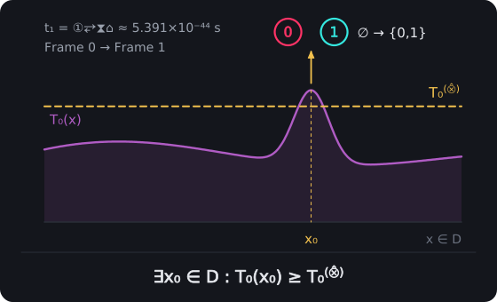
Prime Pulse Activation G

S_0(x_0) → S_1(x_0) via T: {∅} → {0,1} bifurcation [∅]

Where:

• S_0(x_0) [∅] - Zero Substrate state at position x_0
• S_1(x_0) [∅] - dynamic state at position x_0
• x_0 [𝕃] - specific position vector
• T [∅] - transformation operator
• {∅} [∅] - empty set (null state)
• {0,1} [∅] - binary state set

➢ Transition from static potential to dynamic computation — the moment time begins where transformation from Zero Substrate state to dynamic state occurs through Prime Pulse Bifurcation enabling transition from null state to binary computational framework.

Binary Transition Operator

S_1(x) = F[S_0(x), N(x), T_0(x)] [∅]

Where:

• S_1(x) [∅] - dynamic state at position x
• F [∅] - binary transition operator
• S_0(x) [∅] - Zero Substrate state at position x
• N(x) [∅] - neighborhood configuration at position x
• T_0(x) [𝕄·𝕃⁻¹·𝕋⁻²] - initial tension distribution at position x
• x [𝕃] - position vector
• R_d [∅] - recursive depth

Dimensional analysis:
Where (from the book): S_1(x) [∅], F [∅], S_0(x) [∅], N(x) [∅], x [𝕃], R_d [∅]
Read dimensionally: S_1(x) = F(S_0(x), N(x), T_0(x))
[∅]
[∅]([∅], [∅], [𝕄·𝕃⁻¹·𝕋⁻²]) = [∅]
[∅] = [∅] ✓ Valid PulseCore Verified ✓

➢ First computational step establishing recursive depth R_d = 1 — Universe's first calculation where binary transition operator transforms Zero Substrate state using neighborhood configuration and initial tension distribution to create dynamic computational state.

This establishes recursive depth R_d = 1 [∅] as the first instantiation of computational dynamics, connecting directly to quantum indeterminacy mechanisms from Part 5.2. Loop quantum gravity's view (Rovelli, 2004) that geometry emerges from discrete quantum states supports such pre-metric, relational states.

The Critical Tension Condition, Prime Pulse Activation equation, and Binary Transition Operator equation establish how Critical Transition from Frame 0 to Frame 1 functions through cosmic ignition threshold, the moment time begins, and Universe's first calculation, demonstrating initialization requirement where static tension exceeds critical threshold to enable Prime Pulse Activation at t = ①⥂⧗⌂ = 2 × ①⥂⧖⌂ while transformation from Zero Substrate to dynamic state occurs through Prime Pulse Bifurcation.

This provides fundamental activation mechanism where binary transition operator uses neighborhood configuration and initial tension distribution to create recursive depth R_d = 1, enabling the first full Pulse cycle that triggers initial Prime Pulse Bifurcation and establishes recursive computational dynamics from static substrate conditions within spatial domain.

Neighborhood Interactions and Information Architecture

By examining the Neighborhood Definition and Interaction Weight Function we can understand how cosmic social network operates through local coupling structure determining substrate connectivity using interaction radius to establish computational locality, while computational influence networks operate through exponentially decaying interaction weights implementing locality using spatial separation and interaction decay length.

Neighborhood Definition

N(x) = {y ∈ D | ||x - y|| ≤ r_0} [𝕃³]

Where:

• N(x) [𝕃³] - neighborhood around position x
• y [𝕃] - position vectors within domain
• D [𝕃³] - spatial domain
• x [𝕃] - reference position vector
• ||x - y|| [𝕃] - Euclidean distance between positions
• r_0 [𝕃] - interaction radius establishing Computational Locality

➢ Local coupling structure determining substrate connectivity — cosmic social network where neighborhood around position includes all points within interaction radius establishing computational locality for substrate interactions.

Margolus' physics-like models of computation (Margolus, 1984) emphasize such locality-limited coupling where update rules are constrained by nearest-neighbor interactions.

Interaction Weight Function

W(x,y) = w_0 × exp(-||x-y||²/σ_0²) [∅]

Where:

• W(x,y) [∅] - interaction weight between positions x and y
• w_0 [∅] - coupling strength parameter
• x, y [𝕃] - position vectors
• ||x-y|| [𝕃] - spatial separation distance
• σ_0 [𝕃] - Interaction Decay Length (G)
• exp [∅] - exponential function

Dimensional analysis:
Where (from the book): W(x,y) [∅], w_0 [∅], x, [𝕃], ||x-y|| [𝕃], σ_0 [𝕃], exp [∅]
[∅]
[∅] × [∅]([𝕃²] ÷ [𝕃²]) = [∅] × [∅]([∅]) = [∅] × [∅] = [∅]
[∅] = [∅] ✓ Valid PulseCore Verified ✓

➢ Exponentially decaying interaction weights implementing locality — computational influence networks where coupling strength decreases exponentially with spatial separation according to interaction decay length establishing local computational connectivity.

The Neighborhood Definition and Interaction Weight Function establish how cosmic social network functions through local coupling structure that determines substrate connectivity and computational influence networks through exponentially decaying interaction weights that implement locality, demonstrating set-theoretic framework where neighborhood around position includes all points within interaction radius while coupling strength decreases with spatial separation according to interaction decay length.

This provides computational locality constraints that limit substrate interactions to nearest-neighbor coupling for maintaining local information processing architecture, ensuring nearest-neighbor dominance in computational processing while maintaining exponential falloff for distant interactions through local computational connectivity constraints for substrate architecture.

Information Content and Computational Capacity

Zero Substrate contains finite information capacity determining all subsequent computational evolution. By examining the Initial Information Content equation, Total Information Conservation equation, and Kolmogorov Complexity Bound we can understand how cosmic information budget operates through finite information resources for all subsequent evolution determined by possible tension states at each position, while cosmic bookkeeping principle operates through total information conservation throughout recursive dynamics maintaining equality between total and initial information content.

The cosmic computability theorem operates through computational complexity bounds ensuring algorithmic decidability using domain cardinality and tension complexity summation, providing fundamental tractability guarantees that prevent algorithmic undecidability and ensure finite computational resources can describe substrate initialization while maintaining information conservation throughout recursive evolution.

Initial Information Content

I_0 = Σ_x log_2(|T_0(x)|) · ℨᵇ [1ᵇ]

Where:

• I_0 [1ᵇ] - initial information content
• Σ_x [∅] - summation over all positions x
• log_2 [∅] - logarithm base 2 function
• |T_0(x)| [∅] - number of possible tension states at position x
• x [𝕃] - position vector

Dimensional analysis:
Where (from the book): Σ_x [∅], log_2 [∅], |T_0(x)| [∅], x [𝕃]
Read dimensionally: I_0 = log_2(|T_0(x)|) · ℨᵇ
[1ᵇ]
[∅]([∅]) × [1ᵇ] = [∅] × [1ᵇ] = [1ᵇ]
[1ᵇ] = [1ᵇ] ✓ Valid PulseCore Verified ✓

➢ Finite information resources for all subsequent evolution — cosmic information budget where initial information content represents total computational resources available through summation of possible tension states across all spatial positions.

Total Information Conservation

I⊚ = I_0 = I▱ + Iℜ [1ᵇ]

Where:

• I⊚ [1ᵇ] - total information content
• I_0 [1ᵇ] - initial information content
• I▱ [1ᵇ] - substrate information content
• Iℜ [1ᵇ] - recursive information content

Dimensional analysis:
Where (from the book): I⊚ [1ᵇ]
[1ᵇ]
[1ᵇ]
[1ᵇ] + [1ᵇ] = [1ᵇ]
[1ᵇ] = [1ᵇ] = [1ᵇ] ✓ Valid PulseCore Verified ✓

➢ Total information conservation throughout recursive dynamics — cosmic bookkeeping principle where information conservation maintains total content equal to initial content through partitioning between substrate and recursive components.

Initial information provides computational resources for all subsequent evolution, maintaining Information Conservation. Verlinde's entropic gravity proposals (Verlinde, 2011) mirror this conservation, where spacetime dynamics emerge from underlying informational degrees of freedom.

Kolmogorov Complexity Bound

K(S_0) ≤ log_2(|D|) + Σ_x K(T_0(x)) [1ᵇ]

Where:

• K(S_0) [1ᵇ] - Kolmogorov complexity of Zero Substrate
• K [1ᵇ] - Kolmogorov complexity function
• S_0 [∅] - Zero Substrate
• log_2 [∅] - logarithm base 2 function
• |D| [∅] - cardinality of domain D
• Σ_x [∅] - summation over all positions x
• K(T_0(x)) [1ᵇ] - Kolmogorov complexity of tension at position x
• T_0(x) [𝕄·𝕃⁻¹·𝕋⁻²] - static tension at position x

➢ Computational complexity bounds ensuring algorithmic decidability — cosmic computability theorem where Kolmogorov complexity of Zero Substrate remains bounded by domain cardinality plus summation of tension complexities ensuring computational tractability.

Wolfram's digital physics frameworks (Wolfram, 2002) demonstrate how simple local laws generate rich emergent complexity, resonating with these discrete initialization rules.

The Initial Information Content equation, Total Information Conservation equation, and Kolmogorov Complexity Bound establish how cosmic information budget, cosmic bookkeeping principle, and cosmic computability theorem function through finite information resources, total information conservation, and computational complexity bounds, demonstrating logarithmic scaling where tension states contribute to initial information content while conservation laws ensure information equality through substrate and recursive partitioning.

This provides fundamental resource constraints and tractability guarantees where Zero Substrate complexity remains bounded by domain cardinality and tension complexities, ensuring computational evolution preserves information resources while preventing algorithmic undecidability and maintaining finite computational description of substrate initialization throughout recursive dynamics.

Conservation Laws and Physical Emergence

Several quantities remain invariant from Zero Substrate through all subsequent evolution. By examining the Linear Response Function we can understand how cosmic stability principle operates through linear response analysis ensuring substrate stability using Green's Function and tension perturbations.

Conservation Laws (G) include:

• Total Information: I⊚ = I_0 = constant [1ᵇ]
• Topological Charge: Q⧝ = Σ_x sign(det(∇ T_0(x))) = constant [∅]
• Energy-Momentum: E_0 + p_0×𝒞→ = constant [𝕄·𝕃²·𝕋⁻²] (in emergent spacetime)
• Substrate Volume: V_0 = |D| = constant [𝕃³] (discrete lattice sites)

Linear Response Function

δS_1(x) = Σ_y G_0(x,y) × δT_0(y) [∅]

Where:

• δS_1(x) [∅] - perturbation response at position x
• Σ_y [∅] - summation over all positions y
• G_0(x,y) [𝕄⁻¹·𝕃·𝕋²] - Green's Function for substrate response
• δT_0(y) [𝕄·𝕃⁻¹·𝕋⁻²] - tension perturbation at position y
• x, y [𝕃] - position vectors

Dimensional analysis:
Where (from the book): δS_1(x) [∅], Σ_y [∅], G_0(x,y) [𝕄⁻¹·𝕃·𝕋²], δT_0(y) [𝕄·𝕃⁻¹·𝕋⁻²], x, [𝕃]
Read dimensionally: δS_1(x) = G_0(x,y) × δT_0(y)
[∅]
[𝕄⁻¹·𝕃·𝕋²] × [𝕄·𝕃⁻¹·𝕋⁻²] = [∅]
[∅] = [∅] ✓ Valid PulseCore Verified ✓

➢ Linear response analysis ensuring substrate stability — cosmic stability principle where perturbation response depends on Green's Function for substrate response multiplied by tension perturbations across all spatial positions.

The Linear Response Function establishes how cosmic stability principle functions through linear response analysis that ensures substrate stability, demonstrating perturbation response dependence on Green's Function for substrate response multiplied by tension perturbations, providing fundamental stability guarantees for Zero Substrate architecture against small perturbations through linear response theory that maintains computational integrity across spatial positions.

Physical Analogies and Cosmological Implications

By examining the Physical Analogies and Cosmological Implications we can understand how Zero Substrate corresponds to established physical concepts including quantum vacuum through static tension fields, spacetime manifold through lattice geometry, and cosmic inflation through first Pulse propagation, while Pre-Geometric Phase Characteristics establish spatial structure without temporal dynamics and topological invariants that determine computational capacity.

Zero Substrate exhibits direct correspondences to established physical concepts:

Pre-Geometric Phase Characteristics include:

• Spatial structure existing without temporal dynamics
• Geometric relationships preceding temporal evolution
• Topological Invariants (G) establishing structural constraints
• Information content determining computational capacity

The Physical Analogies and Cosmological Implications establish how Zero Substrate functions as computational foundation for physical emergence, demonstrating direct correspondences between substrate components and established physical concepts where static tension fields mirror quantum vacuum states, lattice geometry provides spacetime manifold analog, and metastable substrate states correspond to false vacuum configurations, while Pre-Geometric Phase Characteristics ensure spatial structure exists before temporal evolution with topological invariants establishing structural constraints and information content determining computational capacity for subsequent dynamic evolution.

Chapter 5 Review

Binary Pulse Theory establishes a comprehensive computational framework grounding physical reality in discrete binary operations while preserving essential features of modern physics. The progression through five interconnected explorations reveals how Prime Pulse Bifurcation, {∅} → {0,1} gives rise to the full spectrum of physical phenomena from quantum mechanics to cosmological cycles.

BPT's deepest claim about reality is this: there is only one computational grid, and we are all patterns within it. What appears as separate Universes, dimensions, or realities are simply different viewing perspectives on the same infinite computational substrate. Every conscious being, every particle, every force, and every law of physics emerges from binary dynamics of this single, pixelated grid. We do not inhabit separate realities — we are all interconnected patterns sharing the same fundamental substrate, experiencing it from different harmonic levels and zoom perspectives.

Foundational Architecture

Part 5.1 established the ontological foundation, proposing that the Binary Substrate (G) constitutes reality itself rather than external simulation. Elementary Binary Units (G) operating through discrete Pulse Rhythm intervals create fabric from which spacetime, matter, and physical laws emerge through collective computational behavior. Wheeler's "it from bit" vision (Wheeler, 1989)¹ receives concrete mathematical expression through Shannon's information theory (Shannon, 1948)⁵, while maintaining strict Information Conservation.

Discovery: Instead of Planck time being a given constant, it emerges from more fundamental binary operations — which would account for why t_P has its specific value. Computational Locality ensures state evolution follows strictly local recursive rules with finite propagation speeds emerging naturally from computational constraints, consistent with relativistic principles (Rovelli, 2018).

Quantum Mechanical Emergence

Part 5.2 presented quantum mechanics as a natural emergence from computational phase dynamics rather than fundamental probabilistic postulates. Quantum Indeterminacy becomes Phase Ambiguity in recursive systems operating at computational resolution limits. Quantum Entanglement (G) emerges from shared Recursive Coherence (G) through common computational ancestry rather than nonlocal action, consistent with Bell inequality experiments (Aspect et al., 1982).

Key Result: The Heisenberg Uncertainty Principle (G) derives from Minimum Recursive Resolution (G) R⥥ = ①⥂⧖⌂/①⥂⧗⌂ = 1/2 of substrate, while Wave-Particle Duality (G) represents regime transitions between coherent and localized Pulse configurations. Decoherence (G) results from Environmental Recursive Density (G) forcing phase resolution rather than mysterious wavefunction collapse, aligning with Zurek's decoherence formalism (Zurek, 2003).

Thermodynamic Reinterpretation

Part 5.3 reconceptualized entropy as Phase Drift (G) within recursive binary Pulse systems. Boltzmann's microstate formalism (Boltzmann, 1877) transforms into deterministic desynchronization measures between binary state transitions. Computational Entropy (G) S☫ = -Σ C_{ij} ln(P_{ij}) captures phase misalignment rather than statistical disorder.

Entropy isn't death — BPT reads it as cosmic evolution. The Universe doesn't decay toward heat death; it evolves toward computational renewal. The framework establishes direct correspondences between classical thermodynamics and BPT computational measures, where temperature becomes Recursive Tension Density, heat flow becomes Phase Drift Propagation, and free energy becomes available computational capacity.

Cosmological Renewal

Part 5.4 reframed entropy as Cosmic Renewal Engine rather than termination process. Maximum entropy becomes Computational Null State triggering cyclical regeneration through Frame Transition (G) operations rather than irreversible heat death, supporting cyclic cosmology models (Baum & Frampton, 2007).

Renewal Transformation Operator R implements transitions from maximum entropy null states to renewed low-entropy configurations while preserving total information through Topological Encoding (G). Energy-Information Equivalence maintains thermodynamic consistency across renewal cycles, transforming classical cosmological inevitability into computational renewal protocol.

Primordial Foundation

Part 5.5 completed the theoretical foundation by examining Zero Substrate — pre-temporal computational state from which all reality emerges. Frame 0 (G) exists in temporal stasis ∂S_0/∂t = 0 while containing all structural information necessary for subsequent evolution through Static Tension Vectors, Geometric Constraints, and Potential Energy Fields.

Origin Proposal: The critical transition from Frame 0 to Frame 1 (G) occurs when static tension exceeds critical thresholds T_0(x_0) ≥ T_0^{(⨶)}, triggering Prime Pulse Activation and establishing the first computational cycle. Conservation Laws (G) including Total Information, Topological Charge, and Energy-Momentum remain invariant throughout all subsequent evolution.

Theoretical Integration

The computational substrate framework provides unified foundations connecting quantum mechanics, thermodynamics, and cosmology within a single mathematical structure. In this framework, open questions in modern physics — from quantum measurement to cosmic fine-tuning — appear as natural consequences of computational substrate dynamics rather than puzzles requiring exotic explanations.

Recursive State Evolution S(n+1) = F[S(n), H(n), ℜₙ] governs transitions at every scale from elementary binary units to dimensional emergence. Phase Relationships drive all dynamics whether describing quantum coherence, entropic drift, or renewal mechanisms. Scale Emergence enables collective behavior of discrete binary units to produce continuous physical phenomena through statistical averaging and coherent organization.

Unification

The framework draws on key insights from digital physics approaches by Wolfram (Wolfram, 2002) and Zuse (Zuse, 1969)⁴, quantum computational frameworks by Lloyd (Lloyd, 2006)⁶ and Feynman (Feynman, 1982)⁹, and mathematical Universe hypotheses by Tegmark (Tegmark, 2008)². String-theoretic insights from Polchinski (Polchinski, 1998) suggest potential high-energy extensions, while discrete quantum approaches by Gisin (Gisin, 2022)⁷ and Hardy (Hardy, 2005)⁸ support experimental accessibility of substrate signatures.

Discoveries Summary:

• Modular Coherence Law: (n+1)² mod n = 1 reveals why quantum systems maintain synchronization across scales through mathematical necessity
• Computational Physics Foundation: proposes that reality emerges from discrete binary operations, making the Universe literally a cosmic computer
• Quantum Emergence from Computation: proposes that probabilities emerge from computational phase relationships, offering a reading of the measurement problem
• Entropy as Phase Evolution: reframes entropy as computational evolution rather than decay, enabling cyclical cosmic regeneration
• Zero Substrate Architecture: offers an account of the "something from nothing" problem through computational logic

Empirical Predictions

The theoretical framework generates specific testable predictions across multiple domains:

• Quantum Scale: Discrete energy signatures in ultra-high precision spectroscopy showing temporal quantization effects with ①⥂⧖⌂ = ①⥂⧗⌂/2 periodicity.
  
• Thermodynamic Scale: Discrete entropy jumps during phase transitions corresponding to critical threshold crossings, and spatial entropy correlations following substrate lattice topology with predictable correlation lengths.
  
• Cosmological Scale: Periodic cosmic microwave background fluctuations with period T⟳ reflecting cyclical renewal signatures, and discrete fundamental constant variations during renewal transitions detectable in precision measurements.
  
• Substrate Scale: Preferred spatial directions from substrate anisotropy, and information density bounds I_0/V_0 verifiable through black hole entropy and holographic principle experiments.

Philosophical Implications

Binary Pulse Theory reframes reality's fundamental nature by grounding physical existence in computational processes. The framework suggests consciousness, biological evolution, and complex systems represent natural extensions of the same recursive dynamics governing physics at the most fundamental level.

Zero Substrate provides computational origin for physical laws and constants, while Cyclical Renewal (G) through entropy-driven regeneration offers a possible approach to cosmological fine-tuning problems. Information becomes conserved foundation underlying both physical and abstract phenomena, connecting insights from information theory (Shannon, 1948)⁵ to fundamental physics.

BPT offers a computational account of the hard problem of consciousness, reframes entropy as evolution rather than decay, and proposes a computational foundation for quantum mechanics.

Future Directions

The computational substrate framework opens new research avenues in fundamental physics, complexity science, and consciousness studies. High-energy experiments may detect substrate signatures at Planck scales, while precision measurements could reveal discrete temporal quantization effects and phase relationships in quantum systems.

Cosmological observations may identify renewal signatures in cosmic microwave background patterns and large-scale structure correlations. The framework's extension to biological systems and consciousness could provide computational foundations for understanding life and awareness as natural emergent phenomena rather than mysterious additions to physical reality.

This understanding reframes all apparent separations — between mind and matter, quantum and classical, local and cosmic — as computational perspectives on a single underlying grid. We are not separate observers of reality; we are reality computing itself into awareness through recursive binary dynamics.

The integration of thermodynamic insights from Tolman (Tolman, 1934)²², information-theoretic principles from Shannon (Shannon, 1948)⁵, and gravitational emergence concepts from Verlinde (Verlinde, 2011) suggests rich connections between BPT and established physics warranting further theoretical and experimental investigation.