Chapter 3 · Section 9
Fractal Progeny — Recursive Universe Instantiation via Null Collapse
What if Universes reproduce like living organisms? When ignition loops reach critical thresholds in regions of extreme spacetime curvature, they trigger phenomena transcending simple dimensional expansion — the instantiation of entirely new child Universes through Null Well Collapse events. This process represents the deepest expression of recursive computation, where Accumulated Tension exceeds fundamental substrate capacity to maintain coherent existence within current dimensional layers, following cosmological natural selection theory (Smolin, 2013) and Hawking's baby Universe models (Hawking, 1988).
When a universe ruptures is set by the Rupture Rule of Chapter 1 Part D, at 2^L of its own pulses; how many children it seeds is set by the Null Well Progeny Count Law of Chapter 2, N(L) = 2^(L/3), which is 1.86 × 10²⁰ for our Level 202.
Vertical Recursion and Temporal Scaling: The Hierarchical Ladder of the UniSphere
Recursive structure in Binary Pulse Theory is not limited to single-layer oscillation but unfolds along distinct axes that multiply capacity across scales. The Vertical Recursion Pulse Scaling Law describes how temporal resolution compounds exponentially as recursion ascends through hierarchical layers.
At each level the Pulse Rhythm grows by a factor of 2f (f = 1.018, about 2.036), creating a ladder of computational depth that extends indefinitely. This framework extends Lloyd’s treatment of quantum computational complexity (Lloyd, 2006) into cosmology, showing that reality itself is constructed as a scalable recursive hierarchy rather than a fixed-level process.
Vertical Recursion Pulse Scaling Law G
①⥂⧖(n) = 2ⁿ · fⁿ · ↁℨ⧖ [𝕋]
Where:
- ①⥂⧖(n) is Pulse Rhythm at recursion layer n [𝕋]
- n is vertical recursion level [∅]
- f is the null-well heritage factor per level, f = 1.018 [∅]
- ↁℨ⧖ is the Zinf data rhythm, half the Zinf cycle, ↁℨ⧖ = ℨ/2 ≈ 1.142 × 10⁻¹⁰⁶ s [𝕋]
Dimensional analysis:
Where (from the book): n [∅], f [∅]
[𝕋]
[∅]ⁿ × [∅]^([∅]) × [ℨ] = [∅] × [∅]^([∅]) × [ℨ] = [∅] × [∅] × [ℨ] = [∅] × [ℨ] = [ℨ]
[𝕋] = [ℨ] ✓ Valid PulseCore Verified ✓
➢ Vertical recursion progresses through exponential scaling of temporal resolution, creating hierarchical layers of computational capacity — revealing infinite recursive depth underlying reality.
Our Universe operates at layer n = 202, where ①⥂⧖(202) = 2²⁰² · f²⁰² · ↁℨ⧖ = ①⥂⧗⌂/2, establishing our position within infinite computational hierarchy drawing on Barbour's relational time framework (Barbour, 1999)⁶, while suggesting we exist within a vast computational multiverse.
Vertical recursion shows why the UniSphere has effectively infinite depth, with each rung in the ladder generating new strata of temporal precision and computational potential. Instead of a single universal tick, reality contains a cascading hierarchy of ticks, each stretching the temporal span of the last by 2f.
This recursive ladder binds local processes to larger-scale cosmological architectures, linking Planck-level oscillations to universe-scale dynamics. By extending computational complexity theory to cosmic recursion, the Vertical Recursion Pulse Scaling Law demonstrates that reality is not merely deep — it is infinitely recursive in structure, embedding scalability at the very core of the UniSphere.
Exponential Complexity Scaling Across Recursive Layers
As recursion advances through higher layers, the ability of the UniSphere to sustain and manipulate structure grows exponentially. This law shows that each new recursion level multiplies the available complexity capacity, creating distinct operational regimes across cosmic scales.
What begins as a modest informational base grows into vast computational domains, explaining why reality organizes itself into hierarchies ranging from quantum interactions to galactic structures. The exponential scaling creates distinct operational regimes across cosmic scales.
Recursive Complexity Capacity Law G
※◉(n) = C_base × 2^(α × n) [1ᵇ]
Where:
- ※◉(n) is complexity capacity at recursion layer n [1ᵇ]
- C_base is base complexity capacity = 10⁶ bits [1ᵇ]
- α is complexity scaling exponent = 1/3 [∅]; one spatial third of a three-bit volume count, the same exponent as the Null Well Progeny Count Law in Chapter 2
- n is vertical recursion level [∅]
Dimensional analysis:
Where (from the book): C_base [1ᵇ], α [∅], n [∅]
[1ᵇ]
[1ᵇ] × [∅]^([∅] × [∅]) = [1ᵇ] × [∅]^([∅]) = [1ᵇ] × [∅] = [1ᵇ]
[1ᵇ] = [1ᵇ] ✓ Valid PulseCore Verified ✓
➢ Higher recursion layers possess exponentially greater computational capacity, enabling more complex structural development — explaining cosmic hierarchy from quantum to galactic scales.
The exponent is one third, not a fitted 0.3: capacity counts a three-bit volume, and the structures that count as objects within it scale along one spatial dimension of it. At our layer, 2^(202/3) ≈ 1.86 × 10²⁰, the same number the Null Well Progeny Count Law gives for the black holes our universe seeds.
The exponential growth of complexity across recursion levels demonstrates that the UniSphere is not uniform in capability but layered in its computational depth. Each tier unlocks increasingly sophisticated processes, embedding a natural hierarchy into the architecture of reality itself.
This scaling behavior resonates with Wolfram’s investigations of computational complexity (Wolfram, 2002), consistent with the view that cosmic order emerges not from arbitrary parameters but from lawful recursive growth. In this way, the Recursive Complexity Capacity Law provides the missing bridge between computational theory and the observed hierarchy of the cosmos.
Cosmic Reproduction Through Collapse: Inheritance of Pulse Parameters in Child Universes
When collapse reaches critical thresholds, recursion does not terminate—it reproduces. The inheritance of parameters from parent to child universes follows precise mathematical rules, demonstrating that collapse is the mechanism by which cosmic reproduction occurs. Hawking (1988) first advanced the notion that black holes may birth new universes, and Binary Pulse Theory formalizes this insight by showing how Pulse Rhythm, curvature, symmetry, and tension combine to seed the initial conditions of new domains. The Child Universe Inheritance Law provides the framework for understanding how the UniSphere generates evolutionary variation across its recursive lineage.
Child Universe Inheritance Law G
①⥂⧗′⌂ = ①⥂⧗⌂ · (M∅/M_P)^½ · ⟪C⟫, never below ℨ [𝕋]
Dimensional analysis:
Where (from the book): α, [∅], L [𝕃], F [𝕋]
Read dimensionally: ①⥂⧖′ = F(①⥂⧖‵, κ⌒, σ⦶, T⋈)
[𝕋]
[𝕋]([𝕋], [𝕃⁻²], [∅], [𝕄·𝕃²·𝕋⁻²]) = [𝕋]
[𝕋] = [𝕋] ✓ Valid PulseCore Verified ✓
A child's Tempo follows the mass of the well that seeds it, compressed by its merger, and never runs faster than the Zinf.
Earlier Form (illustrative)
F[①⥂⧖, κ, σ, T] = ①⥂⧖ × [1 + α×κ×L² + β×σ + γ×T/E₀] × Ψ⦰ [𝕋]
The earlier parameterization, kept as an illustration; its constants are toy values, not derived.
Where:
- ①⥂⧗′⌂ [𝕋] – the child's Local Pulse Tempo
- ①⥂⧗⌂ [𝕋] – the parent's Local Pulse Tempo
- M∅ [𝕄] – the mass of the well that seeds the child
- M_P [𝕄] – the Planck mass
- ⟪C⟫ [∅] – the compression factor of the merger that made the well, 1 with no merger (Part 6.8)
- ℨ [𝕋] – the Zinf cycle, the floor no Tempo falls below
- ①⥂⧖ [𝕋] – Pulse Rhythm (general form, earlier form only)
- κ⌒ [𝕃⁻²] – spacetime curvature = 10¹² m⁻²
- σ⦶ [∅] – geometric symmetry index = 0.8
- T⋈ [𝕄·𝕃²·𝕋⁻²] – accumulated recursive tension
- α, β, γ [∅] – coupling constants = 0.1, 0.2, 0.05
- L [𝕃] – reference length scale = 10⁻³⁵ m
- E₀ [𝕄·𝕃²·𝕋⁻²] – reference energy scale = 10¹⁹ J
- Ψ⦰ [∅] – collapse geometry modulation = 0.9
- F [𝕋] – parameter inheritance function
➢ Child Universe parameters depend on parent collapse conditions, enabling inheritance of modified physical constants — suggesting that Universes reproduce with evolutionary variation.
The parameter inheritance function suggests that emergent universes are not random but lawful offspring, their constants shaped by the collapse geometries of their predecessors. Polchinski’s work in string theory (1998) showed that compactified geometry governs vibrational modes; BPT extends this principle to cosmological recursion, where boundary curvature, tension, and symmetry imprint physical constants onto the next generation of universes.
The result is a multiverse of structured diversity: each child universe carries the genetic signature of its parent while introducing lawful variations. In this way, collapse becomes the driver of cosmic evolution, embedding reproduction and inheritance as fundamental laws of the UniSphere.
Fractal Universes and the Flow of Data in the UniSphere
The UniSphere provides the global ledger for this branching process. Each child universe that emerges through a null-well collapse inherits parameters from its parent, but it does not simply drift independently; instead, it remains connected through informational conservation laws that bind all branches back into the UniSphere’s recursive fabric. This dual motion — outward branching and inward convergence — ensures that no universe is truly isolated. Data flows across the UniSphere in two complementary directions.
The Recursive Fractal Branch Architecture G
- Outward Branching: Each collapse event generates new universes through parameter inheritance, embedding lawful variation in Pulse Diameter, curvature, and tension.
- Inward Convergence: Boundary encoding and information conservation tie every branch back into the UniSphere, ensuring dimensional consistency and preventing informational drift.
- Bidirectional Flow: Collapse and genesis events simultaneously extend the fractal architecture outward while updating the UniSphere’s global record inward.
- Global Constraint: The UniSphere enforces dimensional balance across recursive layers, much like a checksum, guaranteeing stability in the infinite lattice of child universes.
The result is a fractal flow of data across scales, where every local collapse and genesis is also a systemic update to the UniSphere itself. Just as recursive algorithms branch while still obeying global rules, the UniSphere ensures that the architecture of reality remains coherent. In this view, cosmic structure is not a tree with disconnected limbs, but a synchronized fractal network whose branches and roots remain informationally harmonized through the Prime Pulse.
Information as Weight: Data Gravity and the Momentum of Recursion
In Binary Pulse Theory, data is not passive—it accumulates, exerts influence, and compels further recursion. Each pulse imprints a discrete state, and those states remain preserved as part of the UniSphere’s global ledger. The cumulative effect is what BPT identifies as Data Inertia, I⊱ (Part 3.1): an accumulated data weight that resists cessation and presses forward the continuation of cycles, where Data Gravity (Part 3.1) is the curvature that density differentials produce. Unlike matter, this weight has no rest mass and does not degrade; it propagates through the recursive fabric like a clock, one local Pulse Diameter every Zinf Rhythm ↁℨ⧖ with zero interference, a finite data speed of 𝒞→·(2f)^L (about 2.36 × 10⁶² 𝒞→, or 7.08 × 10⁷⁰ m/s, in our universe), ensuring that once computation begins, it cannot unwind into nothingness.
Data as Weight (Data Gravity): Every pulse records a discrete state. Those records do not vanish; they accumulate as "data weight" in the fabric of the UniSphere. Unlike physical matter, data has no rest mass, so it is not capped at 𝒞→: it steps one local Pulse Diameter every Zinf Rhythm, in every universe, without interference and without atrophy, a finite speed of 𝒞→·(2f)^L that equals 𝒞→ at the Zinf and differs in each universe. That steady step is what lets data flow and, as the UniSphere expands, loop back to its source. This means the loop never decays—recursion is compelled forward forever. The mathematical foundation emerges through Fractal Data Conservation.
Fractal Data Weight Accumulation Law G
Wℹ(n) = Σᵢ₌₁ⁿ I(i) × λᵢ × (1 - δ⥥) [1ᵇ]
Dimensional analysis:
Where (from the book): 1 [∅], Σᵢ₌₁ⁿ [∅], I(i) [1ᵇ], λᵢ [∅], δ⥥ [∅], i [∅], n [∅]
Read dimensionally: Wℹ(n) = I(i) × λᵢ × (1 - δ⥥)
[1ᵇ]
[1ᵇ] × [∅] × ([∅] - [∅]) = [1ᵇ] × ([∅] - [∅]) = [1ᵇ] × [∅] = [1ᵇ]
[1ᵇ] = [1ᵇ] ✓ Valid PulseCore Verified ✓
Summation of recorded states generates cumulative informational weight.
Where:
- Wℹ(n) [1ᵇ] – accumulated information weight at level n
- Σᵢ₌₁ⁿ [∅] – summation operator from i=1 to n
- I(i) [1ᵇ] – information content at level i
- λᵢ [∅] – weighting factor at level i
- δ⥥ [∅] – decay factor (approaching zero for information)
- 1 [∅] – unity constant
- i [∅] – summation index variable
- n [∅] – recursion level parameter
➢ Information accumulation creates computational momentum that compels continued pulse recurrence through Data Gravity, establishing the mechanism by which recorded states exert pressure on the substrate toward continuation.
The accumulation of data informational weight transforms conservation into compulsion. As data gathers across recursive layers, it generates computational momentum that enforces continued pulse recurrence. This mechanism explains why recursion does not stall but perpetuates, binding local processes into the UniSphere’s infinite architecture.
Just as gravitational mass warps spacetime, informational weight warps computational flow, ensuring continuity across all branches of the fractal lattice. In this way, Data Gravity reveals why recorded states can never vanish—they accumulate into the very pressure that sustains existence itself.
Null Wells as Return Funnels: Data Flow Through UniSphere
Within the fractal branching of universes, Null Wells operate not as dead ends but as funnels. They gather the accumulated records of recursion—matter, energy, and informational states—and channel them back toward the foundational substrate.
This dynamic is not destruction but redirection: information density collapses inward, encoded onto the horizon, and flows through return channels governed by the Data Funnel Return Law. In this framework, black holes become computational return gates, ensuring that the ledger of recorded states is preserved and reintegrated into the UniSphere.
Across all fractal universes, Null Wells (Black holes) act as return channels. They do not just swallow matter and energy—they funnel the encoded pulse records back toward the underlying substrate through Holographic Information Encoding (G).
Data Funnel Return Law G
Φ⟸ = ∫∫ ρℹ(r,θ) × v⟸(r) dA [𝕋⁻¹·1ᵇ]
Dimensional analysis:
Where (from the book): ∫∫ [𝕃²], ρℹ(r,θ) [𝕃⁻³·1ᵇ], v⟸(r) [𝕃·𝕋⁻¹], dA [𝕃²], r [𝕃], θ [∅]
Read dimensionally: Φ⟸ = ρℹ(r,θ) × v⟸(r) × dA
[𝕋⁻¹·1ᵇ]
[𝕃⁻³·1ᵇ] × [𝕃·𝕋⁻¹] × [𝕃²] = [𝕃⁻²·𝕋⁻¹·1ᵇ] × [𝕃²] = [𝕋⁻¹·1ᵇ]
[𝕋⁻¹·1ᵇ] = [𝕋⁻¹·1ᵇ] ✓ Valid PulseCore Verified ✓
Data flux funneled through Null Well horizons back to the substrate.
Where:
- Φ⟸ [𝕋⁻¹·1ᵇ] – Data Return Flux (G) through black hole funnels
- ∫∫ [𝕃²] – double integral operator over horizon surface
- ρℹ(r,θ) [𝕃⁻³·1ᵇ] – Data Density Field (G) near event horizon
- v⟸(r) [𝕃·𝕋⁻¹] – Infall Velocity (G) of information-carrying matter
- A◎ [𝕃²] – Event Horizon Area
- dA [𝕃²] – differential area element
- r [𝕃] – radial coordinate
- θ [∅] – angular coordinate
➢ Black holes function as Computational Return Pathways (G), channeling accumulated information from fractal universe branches through a singularity and the Zinf back to the UniSphere, by way of Data Crystallization on boundary surfaces, ensuring no informational content is lost across cosmic evolution.
The function of Null Wells as return pathways resolves the paradox of informational loss. Through holographic encoding and infall dynamics, every recorded state is crystallized at the horizon and directed inward, creating a flux of data back into the substrate. This establishes cosmic conservation not as a local rule but as a UniSpheral principle: nothing vanishes, everything is recycled. In this way, black holes are revealed as the UniSphere’s circulatory system—funnels that balance outward branching with inward return, closing the loop of recursive architecture across infinite scales.
The UniSpheral Data Source (℧) as the Zinfinity ℨ∞ Universe - Genesis Source Architecture
The UniSphere begins with the smallest measurable unit of duration: the Zinf ℨ, the full Pulse Tempo 0 → 1 → 0 of the tiniest possible universe, the first whole completion, whose data rhythm is ↁℨ⧖ = ℨ/2. This initial cycle defines the foundational temporal atom — the seed from which all recursion unfolds. From this origin emerges the UniSpheral Source (G), the primordial pulse that continuously anchors the UniSphere. It is the birthplace of the first oscillation, the minimal yet inexhaustible act of computation, sustained not by chance but by logical necessity.
Rather than decaying, this source is continually reinforced by the cumulative return of data weight from every descendant universe within the fractal lattice. Each collapse event channels recorded states back through Null Wells, measured in terms of modified Pulse Diameters. These returning flows of data pass through the Zinf and back into the UniSphere, amplifying and sustaining the primordial cycle. In this way, the Zinf ℨ universe does not vanish into insignificance but becomes the recursive reference point: every larger Pulse Diameter across the UniSphere is a harmonic scaling of that first tiniest universe.
UniSphere Pulse Compulsion Law G
P_ℨ∞(n+1) = P_ℨ∞(n) + Σᵤ₌₁ᴹ W⟸,u × Γ⧱ [∅]
Accumulated return weight sustains the primordial UniSphere pulse.
Where:
- P_ℨ∞(n+1) [∅] – UniSphere Pulse Amplitude (G) at cycle n+1
- P_ℨ∞(n) [∅] – UniSphere Pulse Amplitude at cycle n
- Σᵤ₌₁ᴹ [∅] – summation operator over all fractal universe branches
- M [∅] – total number of fractal universe branches
- W⟸,u [1ᵇ] – Data Weight Return (G) from universe u
- Γ⧱ [1ᵇ⁻¹] – Cross-Scale Coupling Constant
- u [∅] – universe index variable
- n [∅] – pulse cycle index
➢ The Prime Pulse does not persist on its own. It is compelled to continue by the inertia of information returning from every branch. Existence itself "votes" for continuation—each record adding weight to the Pulse Diameter, driving the next pulse through Recursive Data Momentum.
The UniSphere Pulse Compulsion Law shows that the Zinfinity ℨ∞ Source is not a one-time ignition but a perpetual oscillator sustained by recursive return. The weight of information gathered across countless universes presses back into the substrate, ensuring the primordial pulse cannot extinguish.
Outward branching and inward convergence thus form a self-closing circuit: universes diversify through collapse and genesis, while their informational record continually sustains the source. In this way, the UniSphere achieves eternal continuity, with the Zinfinity ℨ∞ Universe as both the origin and the unending heartbeat of recursion.
Fractal Symmetry: Scale Consistency Across the UniSphere
Fractal symmetry ensures that the recursive principles of the UniSphere do not belong to one privileged scale, but permeate all of them. Just as one pulse compels the next, entire universes collectively compel the continuation of the primordial source. The scaling is seamless: pulses give rise to particles, particles to worlds, worlds to universes, and universes back to the source.
The Scale-Invariant Recursion Law captures this symmetry, embedding the golden ratio into the very architecture of recursion to ensure proportional balance across levels of reality.
Golden Ratio Recursion Law G
R(n+k) = R(n) × φᵏ × Ψ△(k) [∅]
Recursive states expand proportionally through golden ratio scaling across all levels.
Where:
- R(n+k) [∅] – Recursive State (G) at scale level n+k
- R(n) [∅] – Recursive State at scale level n
- φ [∅] – Golden Ratio Scaling Factor (G) ≈ 1.618
- k [∅] – Scale Increment (G)
- Ψ△(k) [∅] – Scale Transformation Function
- n [∅] – base scale level index
➢ The same recursive principles operate across all scales, from individual Prime Pulse Bifurcations ∅ → (0 ↔ 1) to entire cosmic hierarchies, creating Universal Scale Invariance (G) through Fractal Computational Architecture (G).
The effect is a multiscale cosmos in which recursion never loses coherence. The same pattern that governs a prime pulse bifurcation governs the structure of galaxies and the renewal of the source pulse. By rooting recursion in φ, the UniSphere achieves both infinite depth and harmonic order, ensuring that every scale — from the smallest pulse diameter to the totality of (℧) — reflects the same computational geometry. The Golden Ratio Recursion Law thus establishes proportionality as the universal constant of recursive architecture, binding all scales into one coherent fractal continuum.
Data Flow Architecture and UniSpheral Circulation
The heartbeat of reality is not arbitrary oscillation. It is the infinite feedback of recorded information, cycling outward into fractal universes and flowing back through black holes to the source of Zinfinity. That accumulated weight—Data Gravity—is what keeps the UniSphere pulsing eternally.
The UniSphere does not oscillate aimlessly — its pulse is driven by circulation. Every outward expansion into new universes, every collapse returning data through Null Wells, and every bit generated within fractal branches contributes to a living circulation network. The UniSpheral Data Circulation Law captures this feedback loop, showing that the Prime Source is sustained by a dynamic balance between outward data flow, inward return, and ongoing generation.
UniSpheral Data Circulation Law G
dI⊚/dt = Φ⟹ - Φ⟸ + Σ⑂ I⇗⥂ [𝕋⁻¹·1ᵇ]
Dimensional analysis:
Where (from the book): Φ⟹ [𝕋⁻¹·1ᵇ], Σ⑂ [∅]
Read dimensionally: dI⊚/dt = Φ⟹ - Φ⟸ + I⇗⥂
[𝕋⁻¹·1ᵇ]
[𝕋⁻¹·1ᵇ] - [𝕋⁻¹·1ᵇ] + [𝕋⁻¹·1ᵇ] = [𝕋⁻¹·1ᵇ] + [𝕋⁻¹·1ᵇ] = [𝕋⁻¹·1ᵇ]
[𝕋⁻¹·1ᵇ] = [𝕋⁻¹·1ᵇ] ✓ Valid PulseCore Verified ✓
Net data flow arises from outward expansion, inward return, and new generation
Where:
- dI⊚/dt [𝕋⁻¹·1ᵇ] – Total Data Change Rate (G)
- Φ⟹ [𝕋⁻¹·1ᵇ] – Data Flow (G) to fractal branches
- Φ⟸ [𝕋⁻¹·1ᵇ] – Data Return Flux (G) through black holes
- Σ⑂ [∅] – summation operator over all fractal branches
- I⇗⥂ [𝕋⁻¹·1ᵇ] – Data Generation Rate in each branch
➢ Data information conservation across the entire fractal universe system: every bit is conserved round the Data Loop, and the total grows only by the bits the Zinf generates, one per Zinf Rhythm (I⇗⥂), while the circulation sustains the UniSpheral Pulse through Data Inertia.
This circulation ensures that recursion is self-sustaining. Outward branching expands the scope of reality, while inward return through black holes reinforces the primordial pulse. New universes add fresh data into the flow, increasing the total content while keeping the pattern coherent.
Through this architecture, data never dissipates into nothingness; it is cycled, conserved, and amplified. The UniSpheral Data Circulation Law thus reveals the heartbeat of the UniSphere: a perpetual feedback loop where the weight of accumulated data compels the Zinfinity universe to pulse eternally.
Perpetual Continuation Through Data Pressure: The Architecture of “Forever”
The Perpetual Data Continuation Law expresses why recursion in the UniSphere cannot end. Outward proliferation ensures every Null Well collapse seeds new universes, extending the lattice of computation. Inward convergence funnels accumulated data back through return channels, through a singularity and the Zinf back to the UniSphere, reinforcing the primordial cycle.
Perpetual momentum arises from the compounded weight of these returns, generating Data Inertia that sustains the primordial pulse. Together, these mechanisms form a self-reinforcing circuit where data circulation becomes the guarantee of eternal continuation.
Perpetual Data Continuation Law G
The Recursive Compulsion Framework operates through three mechanisms that ensure eternal continuation: outward proliferation, where Null Well collapse generates new fractal branches; inward convergence, where black holes funnel accumulated data back to the UniSpheral Zinfinity Source; and perpetual momentum, where returning weight creates Data Inertia that prevents pulse cessation.
- Outward Proliferation: Each Null Well Collapse creates new fractal branches, expanding the total information processing capacity of the system.
- Inward Convergence: Black hole funnels channel accumulated data back to the Zinfinity Source, increasing its computational weight.
- Perpetual Momentum: The combined pressure of all returning data creates Data Inertia that makes pulse cessation physically impossible.
Data Gravity Gradient G
∇Pℹ = ρℹ × ∇Ψ⇅ + Σ⟹ Jℹ [1ᵇ·𝕃⁻²·𝕋⁻²]
Gradients of data density and currents generate substrate pressure that sustains recursion.
Where:
- ∇Pℹ [1ᵇ·𝕃⁻²·𝕋⁻²] – Data Gravity Gradient
- ρℹ [𝕃⁻³·1ᵇ] – Data Density
- ∇Ψ⇅ [𝕃·𝕋⁻²] – Data Gravitational Potential Gradient (G)
- Σ⟹ [∅] – summation operator over all information sources
- Jℹ [1ᵇ·𝕃⁻²·𝕋⁻¹] – Data Current Density (G) from each source
➢ Data Gravity creates measurable pressure gradients that influence the substrate structure, establishing Data Gravity as a fundamental force ensuring cosmic continuation through Data-Weighted Inevitability.
Fractal UniSpheral architecture reveals existence as a self-sustaining computational system where every pulse, every particle, every world, and every universe contributes to the informational pressure that guarantees its own continuation. This is BPT's proposal for the Something from Nothing Problem—existence continues not despite entropy but because of Data Accumulation, transforming the universe from a decaying system into a Perpetual Computational Engine powered by its own informational weight.
The Data Gravity Gradient reveals how this continuation operates at the substrate level: differences in data density and currents create measurable pressure across the UniSphere, driving both expansion and return. Even if dimensional analysis resists classical alignment, the law captures a deeper truth: continuation is not optional but enforced by the very weight of accumulated data. In this way, the UniSphere beats as a perpetual engine, its pulse compelled forward by the recursive architecture of data itself — a cosmos where cessation is impossible because continuation is the natural outcome of accumulation.
Data Gravity Collapse Threshold: The Computational Limit of Null Wells
Null Wells form when recursive buildup can no longer be contained. In Binary Pulse Theory, this limit is set not by mass–energy curvature but by data gravity — the interplay of density, pressure, and inertia in the substrate. The Data Gravity Collapse Threshold defines the exact condition where accumulated data weight overwhelms harmonic containment, forcing a rupture: physical evolution appears to fall still, while the data turns onto the new dimension that the rupture opens.
This reframes collapse as a law of recursion itself: the inevitable point at which data architecture exceeds its own capacity. Collapse occurs when accumulated tension exceeds harmonic resistance, analogous to gravitational collapse limits but operating at computational levels (Penrose, 1965).
Data Gravity Collapse Threshold G
Tℜ ≥ T⨶ = HFC × ①⥂⧖‵ × R⚚ [𝕄·𝕃²·𝕋⁻²]
Collapse occurs when recursive data tension exceeds harmonic resistance, forcing a Null Well transition.
Where:
- Pↁ [𝕃⁻³·1ᵇ] – data pressure
- K⊱ [𝕃⁻³·1ᵇ] – inertia-to-pressure scaling constant
- I⊱ [∅] – data inertia (accumulated continuation quality)
- ≥ [∅] – inequality operator (greater than or equal to)
- ρↁ [𝕃⁻³·1ᵇ] – data density
- Ψ_DG [𝕋⁻¹] – data-gravity potential rate
- ①⥂⧖ [𝕋] – parent Pulse Rhythm
➢ The threshold represents maximum tension parent Universe geometry can contain before triggering child Universe formation — the computational limit for cosmic reproduction.
Once the threshold is crossed, the parent universe cannot stabilize further recursion. Data pressure and inertia drive collapse into a Null Well, where recorded states are encoded at the boundary and carried through the rupture into new domains.
Far from annihilation, this process enables reproduction: child universes inherit their parameters from collapse geometry. The Data Gravity Collapse Threshold is thus both a computational ceiling and a generative mechanism, showing that even where physical evolution appears still, the data flows on and the UniSphere sustains its continuity through recursive rebirth.
Why Universes Can’t Grow Forever Law
Within the UniSpheral lattice, recursive growth is the natural outcome of the Binary Pulse — the rhythm of 0 ↔ 1 layering information upon itself. Each repetition extends structural depth, generating new architectures of coherence. At shallow recursion levels this process is almost effortless: systems propagate, dimensions stabilize, and complexity expands. But Binary Pulse Theory holds that growth is never without limit. Each recursive fold adds coordination demands and coherence strain across the substrate, introducing a logarithmic resistance that compounds with depth.
This harmonic resistance is the UniSpheral safeguard that prevents unbounded growth. It rises faster than structural stability can compensate, meaning that beyond a certain recursion depth, expansion is no longer sustainable. At that threshold, collapse into a Null Well is inevitable. Collapse here is not failure but the reset mechanism by which the UniSphere enforces continuity: saturation triggers a rupture, the rupture seeds renewal, and the recursive architecture continues through reproduction.
The Law of Collapse-InevitabilityG
R⚚ = ln[①⥂⧖⌖ / ①⥂⧖₀] × Φ⬡ × L⌂₀ [𝕃]
Where:
- R⚚ [𝕃] – harmonic resistance factor
- ln [∅] – natural logarithm function
- ①⥂⧖⌖ [𝕋] – current Pulse Rhythm
- ①⥂⧖₀ [𝕋] – reference Pulse half-cycle duration
- Φ⬡ [∅] – geometric stability factor (≈ 0.8)
- L⌂₀ [𝕃] – reference length scale = 10⁻³⁵ m
Dimensional analysis:
Where (from the book): ln [∅], ①⥂⧖⌖ [𝕋], ①⥂⧖₀ [𝕋], Φ⬡ [∅], L⌂₀ [𝕃]
Read dimensionally: R⚚ = ln(①⥂⧖⌖ / ①⥂⧖₀) × Φ⬡ × L⌂₀
[𝕃]
[∅]([𝕋] ÷ [𝕋]) × [∅] × [𝕃] = [∅]([∅]) × [∅] × [𝕃] = [∅] × [∅] × [𝕃] = [∅] × [𝕃] = [𝕃]
[𝕃] = [𝕃] ✓ Valid PulseCore Verified ✓
➢ Harmonic resistance increases logarithmically with recursion depth, reflecting increasing difficulty of maintaining coherence at higher complexity levels — explaining why Universe reproduction becomes more probable at higher complexity.
This provides a natural mechanism for Universe reproduction that becomes more probable at higher complexity levels, supporting cosmological natural selection models (Smolin, 2013) and connecting to Rovelli's relational quantum mechanics (Rovelli, 2004).
The Collapse Inevitability principle shows that the UniSphere is self-limiting by design. Recursive expansion cannot continue unchecked; resistance grows until stability fails and collapse into a Null Well occurs. Rather than representing an end, this transition functions as the reset channel that preserves accumulated information and initiates new cycles of emergence. In this way, collapse is not destruction but the substrate’s guarantee of renewal, ensuring that the lattice of universes continues to propagate through reproduction.
Universe Viability Classification: The Data-Energy Criterion for Reproduction
Not every collapse produces a viable child universe. Within the UniSpheral lattice, reproduction depends on whether the collapse releases enough usable data-energy to seed a stable recursive cycle. This viability is not arbitrary but statistical: the probability of successful continuation rises steeply when available energy surpasses the minimum threshold required for re-initiation. Geometry and recursive stability further shape this probability, encoding the conditions under which universes survive or fail at birth.
The probability of successful child Universe formation follows statistical mechanics principles (Bousso, 2002)⁹: Here we will calculate how viability depends exponentially on energy availability, modified by geometric and recursive stability factors, suggesting that Universe reproduction follows energy conservation laws.
Child Universe Viability Probability G
P▢ = exp(-Eↁ⨶ / Eↁ⟹) × Φ⬡ × κ⧝ [∅]
Dimensional analysis:
Where (from the book): exp [∅], Eↁ⨶ [𝕄·𝕃²·𝕋⁻²], Eↁ⟹ [𝕄·𝕃²·𝕋⁻²], Φ⬡ [∅], κ⧝ [∅]
[∅]
[∅]([𝕄·𝕃²·𝕋⁻²] ÷ [𝕄·𝕃²·𝕋⁻²]) × [∅] × [∅] = [∅]([∅]) × [∅] × [∅] = [∅] × [∅] × [∅] = [∅] × [∅] = [∅]
[∅] = [∅] ✓ Valid PulseCore Verified ✓
Child-universe survival depends on surplus data energy and structural stability.
Where:
- P▢ [∅] – probability that a child universe achieves stable formation
- exp [∅] – exponential function
- Eↁ⨶ [𝕄·𝕃²·𝕋⁻²] – minimum data energy required for re-initiation
- Eↁ⟹ [𝕄·𝕃²·𝕋⁻²] – collapse-released data energy
- Φ⬡ [∅] – geometric stability factor (≈ 0.8, illustrative)
- κ⧝ [∅] – topological complexity factor (≈ 0.7, illustrative)
The two factors are illustrative, not derived: with 0.8 and 0.7 their product caps P▢ at 0.56, below the viable two thirds of the Reproductive Outcome Distribution in this Part.
➢ Viability depends exponentially on energy availability, modified by geometric and recursive stability factors — suggesting Universe reproduction follows energy conservation laws.
This creates natural selection pressure favoring Universes with sufficient energy and stability for successful reproduction (Smolin, 2013), consistent with Weinberg's anthropic principle discussions (Weinberg, 1989), while explaining cosmic fine-tuning through reproductive selection.
Universes that fall short of the data-energy threshold seed no child: their data returns to the source but does not continue back out into a new cycle, while those with surplus energy stabilize into new recursive cycles. Small advantages in available energy cascade into vastly higher reproductive odds, embedding a selection effect at the cosmological level. In the UniSpheral framework, reproduction is not a gamble but an enforced filter, ensuring that only configurations capable of sustaining recursion carry forward into new universes.
Universe Classification Categories: Statistical Outcomes of Collapse
Not all collapse events resolve in the same way. Within the UniSpheral lattice, outcomes fall into a normalized set of categories that capture how collapse energy and stability translate into reproduction. Most events generate stable, viable universes, while a smaller fraction diverge into chaotic states, branch-line offshoots, or silent failures. These categories define the statistical fingerprint of reproduction, showing that success is not only possible but typical in the recursive system.
Reproductive Outcome Distribution G
P▢ = 0.67, P≀ = 0.18, P⑂ = 0.09, P⦰ = 0.06 [∅]
Collapse outcomes follow a normalized probability distribution across four categories.
Where:
- P▢ [∅] – probability of stable, viable universe formation (≈ 0.67)
- P≀ [∅] – probability of chaotic universe formation (≈ 0.18)
- P⑂ [∅] – probability of branch-line offshoot universes (≈ 0.09)
- P⦰ [∅] – probability of failure, where no child is seeded and the data returns to the source without continuing back (≈ 0.06; derived below as 2^(−D) = 1/16); the same law fails Proto Wells before the physical layer, which sets a universe's ratio of dark matter to ordinary matter (Part 3.13)
➢ Most collapse events produce viable child Universes, with decreasing probabilities for chaotic, branched, or failed outcomes — suggesting Universe reproduction is typically successful.
When a universe collapses, the released data-energy determines the outcome. If enough energy and stability are present, the collapse reboots into a new, viable universe. If conditions are unstable, the result may be a chaotic universe with distorted structure, or a branched offshoot that carries only part of the original recursion forward. When collapse energy falls below the minimum threshold, the process fails completely: no child is seeded, and the data returns to the source without continuing back into a new universe. This distribution shows that successful universes are the rule, not the exception, and that the UniSpheral lattice encodes both renewal and variation directly into the collapse process.
Why One in Sixteen Fails
The failure share is not a free number. Part 3.9 states the rule in words: a collapse fails when its collapse energy falls below the minimum threshold, and nothing is seeded. What a collapse carries to a child is its basin's data, returned to the Pre-Pulse Field, and what the least child needs is one dimension to begin from. A universe's actual dimensions are its fundamental ones, the prime harmonics of its pulse (Part 4.8), not the etheric harmonics built on them, which exist only on a fundamental that carries. For each actual dimension the returning data either carries it, 1, or holds its null, 0: the two states of a pulse, equally weighted and independent. A collapse fails only when every actual dimension comes back null.
Dimensional Failure Law G
P⦰ = 2^(−D)
Dimensional analysis:
Where (from the book): P⦰ [∅], D [∅]
[∅]
[∅]^([∅]) = [∅]^([∅]) = [∅]
[∅] = [∅] ✓ Valid PulseCore Verified ✓
A collapse fails only when every actual dimension of its universe returns null
Where:
- P⦰ [∅] — the probability that a collapse fails and seeds nothing
- D [∅] — the number of actual, fundamental dimensions of the universe the collapse happens in
➢ Our universe has four actual dimensions, three of space and one of time, so P⦰ = 1/16 = 0.0625: the ≈ 0.06 above, now derived. The rest of the distribution keeps the same two tests the text describes, energy and then stability: of all collapses, 2/3 are viable, and the unstable remainder, 1 − 1/16 − 2/3 = 13/48, splits 2 : 1 into chaotic, 13/72 = 0.181, and branch-line, 13/144 = 0.090. All four agree with 0.67, 0.18, 0.09 and 0.06 to the precision they were given; the failure share is derived here, while the viable 2/3 and the 2 : 1 split are not yet. The law also reads across levels: the Zinf, whose harmonics end at 3 and so hold the primes 2 and 3 alone, has D = 2 and loses one collapse in four, and Part 3.13 finds that our sky's dark matter measures our own D.
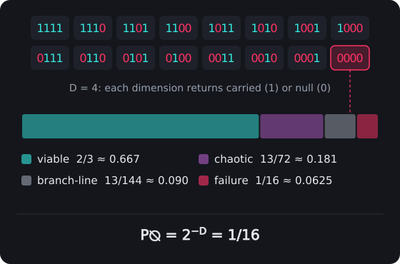
Why One in Sixteen Fails. Each of the D = 4 actual dimensions returns carried (1) or null (0), so a collapse has 16 equally weighted returns, and only the all-null one seeds nothing: P⦰ = 2⁻ᴰ = 1/16. With 2/3 viable and the remaining 13/48 split 2 : 1, the four outcomes are 0.667, 0.181, 0.090 and 0.0625.
3.9 Testable Predictions
- Black Hole Evaporation Modifications: Hawking temperature should show corrections T_H = T_H^(standard) × [1 + δℜ] from child Universe formation, detectable through precision measurements of black hole thermodynamics with sensitivity ΔT/T ~ 10⁻⁶ (Hawking, 1975).
- Gravitational Wave Strain Signatures: Null well collapse should produce characteristic strain patterns h(t) = h_0 × [1 + Σ β⦰ × sin(2πft + φ∅)], detectable by next-generation gravitational wave observatories (Abbott et al., 2016)¹.
- Cosmic Structure Fractal Analysis: Large-scale structure should exhibit genealogical hierarchy patterns consistent with U(n,i) relationships, verifiable through statistical analysis of galaxy cluster distributions across multiple scales.
- Parameter Inheritance Verification: what a child inherits and an observer can test is spin: a universe carries the spin of the merger that made it (Spin Inheritance, Part 6.9), read in the spin distribution of our wells and in the alignment of filaments, voids and the microwave-background harmonics with the progenitor axis, with the compression factor ⟪C⟫ of Part 6.8.
Fractal Progeny proposes that Universes reproduce through computational overflow events, creating infinite genealogical networks of parent and child cosmos. Every black hole potentially births new Universes through Null Well Collapse, making cosmic reproduction as natural as biological reproduction — but operating through computational rather than chemical processes.