Chapter 7 · Section 3
Quantum Mirrors of the Prime Pulse — Interference Patterns as Substrate Echoes
How do quantum interference patterns reveal the underlying computational structure of reality itself? Binary Pulse Theory models physical reality as emerging from recursive binary oscillations between {0,1} states through Prime Pulse Bifurcation mechanisms, where these oscillations form the computational substrate of spacetime and matter established in Parts 5.1-5.5.
Building upon the Harmonic Origin Pulse P(n) = (n+1)² from Part 7.2 and the Recursive Harmonic Spectrum (G) H_n = ν_0 × (n + 1)² from Part 7.1, quantum interference patterns are not purely probabilistic phenomena, but direct echoes of the substrate's recursive architecture operating through Recursive State Evolution and Substrate-Pulse Coupling, consistent with fundamental quantum postulates (Bohr, 1928)⁸. This is how BPT meets Bell's theorem (Bell, 1964) and the loophole-free tests that confirm its violation (Hensen et al., 2015; Giustina et al., 2015; Shalm et al., 2015): no local hidden variables cross space; the correlation comes from the shared loop that all data passes through, the UniSphere and the Zinf; and no message can be sent faster than light, since each observer's result looks random until the results are compared by ordinary means.
Substrate Wave Function Architecture and Interference Formalism
The Substrate Wave Function (G) incorporates both active Pulse states and inactive null regions through tensor product structure. By examining the Substrate Wave Function Architecture and Interference Formalism, we can understand how quantum mechanical tensor product structures encode both active computational processing and inactive null states in binary substrate systems, revealing the mathematical framework for describing interference conditions, coherence evolution, and quantum overlap requirements in recursive computational architectures.
Substrate Wave Function
Ψ▱(x,t) = sum_n c_n |n_p⟩ ⊗ |n_0⟩
Where:
- Ψ▱(x,t) [𝕃⁻³/²] - substrate wave function dependent on position and time
- x [𝕃] - spatial coordinate
- t [𝕋] - temporal coordinate
- sum_n - summation operator over all computational states n
- c_n [∅] - complex amplitude coefficients
- |n_p⟩ [∅] - active Pulse state with n transitions
- n [∅] - number of computational transitions
- ⊗ - tensor product operator
- |n_0⟩ [∅] - inactive/null state region
- [∅] - quantities without physical units, pure numerical ratios or mathematical constants
➢ Tensor product structure encodes both computational activity and pause states in binary substrate, demonstrating how quantum mechanical formalism captures the dual nature of active processing and suspended computation in recursive computational architectures.
Prime Pulse Interference Condition
⟨Ψ_1|Ψ_2⟩ = sum_(n,m) c_1n c_2m ⟨n_p|m_p⟩ ⟨n_0|m_0⟩ [∅]
Where:
- ⟨Ψ_1|Ψ_2⟩ [∅] - inner product represents Prime Pulse Interference Condition
- Ψ_1 [𝕃⁻³/²] - first substrate wave function
- Ψ_2 [𝕃⁻³/²] - second substrate wave function
- sum_(n,m) - double summation operator over computational state indices n and m
- c_1n [∅] - complex amplitude coefficient for first wave function at state n
- c_2m [∅] - complex amplitude coefficient for second wave function at state m
- ⟨n_p|m_p⟩ [∅] - inner product between active pulse states
- ⟨n_0|m_0⟩ [∅] - inner product between inactive null states
- n [∅] - computational state index for first function
- m [∅] - computational state index for second function
- [∅] - quantities without physical units, pure numerical ratios or mathematical constants
➢ Interference requires coherent overlap between Pulse states and null regions, demonstrating how quantum mechanical inner products determine the conditions for constructive and destructive interference in binary computational substrate systems.
Coherence Factor
C(Δt) = |⟨Ψ(t)|Ψ(t+Δt)⟩|² [∅]
Where:
- C(Δt) [∅] - Coherence Factor
- Ψ(t) [𝕃⁻³/²] - substrate wave function at time t
- Ψ(t+Δt) [𝕃⁻³/²] - substrate wave function at time t+Δt
- t [𝕋] - initial time
- Δt [𝕋] - temporal separation
- | |² - squared magnitude operator
- ⟨ | ⟩ - inner product operator
- 0 [∅] - complete decoherence limit
- 1 [∅] - perfect self-coherence value
- ∞ [∅] - infinite time limit
- ①⥂⧗⌂ [𝕋] - Local Pulse Tempo (Planck time), equal to 2 × ①⥂⧖⌂
- ①⥂⧖⌂ [𝕋] - Local Pulse Rhythm time interval
- [∅] - quantities without physical units, pure numerical ratios or mathematical constants
➢ Temporal coherence preservation through Pulse Rhythm time intervals with ①⥂⧗⌂ = 2 × ①⥂⧖⌂ full cycle duration, demonstrating how computational substrate maintains quantum coherence over discrete temporal separations with boundary conditions ranging from perfect self-coherence to complete decoherence.
The Substrate Wave Function Architecture and Interference Formalism demonstrates how Binary Pulse Theory employs quantum mechanical formalism to characterize computational substrate dynamics through tensor product wave functions, interference overlap conditions, and temporal coherence factors that collectively describe the quantum nature of binary computational processing and enable analysis of coherence preservation, decoherence mechanisms, and interference patterns in recursive substrate architectures.
Experimental Manifestations and Substrate Correlations
The framework connects with experimental quantum mechanics through matter-wave interferometry, particularly in demonstrations of wave-particle duality for large molecules (Arndt et al., 1999)⁹. By examining the Experimental Manifestations and Substrate Correlations framework, we can understand how Binary Pulse Theory connects to experimental quantum mechanics through matter-wave interferometry and large molecule demonstrations, revealing the mathematical relationships between substrate correlation lengths, mass scaling, and visibility predictions that enable testable predictions for quantum coherence in computational substrate systems.
C₆₀ Fullerene Parameters:
- Mass: m = 720 amu = 1.196 × 10⁻²⁴ kg
- de Broglie wavelength: λ_dB ≈ 2.5 pm
Substrate Correlation Length
ξ▱ ≈ lₚ (m/mₚ)^(1/3) [𝕃]
Where:
- ξ▱ [𝕃] - substrate correlation length
- lₚ [𝕃] - Planck length
- m [𝕄] - particle mass
- mₚ [𝕄] - Planck mass
- ^(1/3) [∅] - cube root exponent
- [∅] - quantities without physical units, pure numerical ratios or mathematical constants
➢ Correlation length scales with mass through dimensional analysis of substrate correlation requirements, demonstrating how particle mass determines the spatial extent of quantum coherence in computational substrate systems through cube root scaling relationships.
Theoretical Justification for 1/3 Exponent: With the Planck density ρₚ = mₚ/lₚ³ the law reads ξ▱ ≈ (m/ρₚ)^(1/3): the edge of a cube that holds the mass m at the Planck density. A mass spread through d⊹ = 3 dimensions at fixed density has an edge growing as m^(1/d⊹), so the correlation length grows with mass as the cube root: α = 1/3. (The Compton length ħ/mc shrinks as the mass grows; it is not the scale this law describes.)
Visibility Prediction
V☫ = V_0 exp(-m/m≋) [∅]
Where:
- V☫ [∅] - Visibility Prediction
- V_0 [∅] - maximum visibility
- exp - exponential function
- m [𝕄] - particle mass
- m≋ [𝕄] - Substrate Coherence Mass Scale, equal to 10⁶ amu
- 10⁶ [∅] - numerical coefficient
- amu [𝕄] - atomic mass unit
- [∅] - quantities without physical units, pure numerical ratios or mathematical constants
➢ Exponential mass dependence reflects substrate coupling strength scaling with particle complexity, demonstrating how increasing particle mass systematically reduces quantum interference visibility through computational substrate interaction mechanisms.
The Experimental Manifestations and Substrate Correlations framework demonstrates how Binary Pulse Theory provides quantitative predictions for experimental quantum phenomena through correlation length scaling and exponential visibility dependence on particle mass, connecting theoretical computational substrate properties to observable quantum interference effects and enabling experimental verification of recursive substrate architectures through matter-wave interferometry measurements.
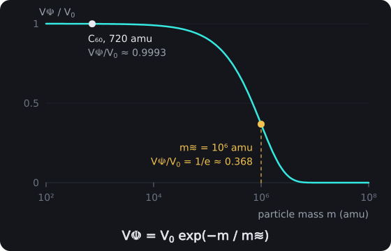
Interference Visibility and Mass. The Visibility Prediction V☫ = V₀ exp(−m/m≋) with m≋ = 10⁶ amu. For the C₆₀ fullerene, m = 720 amu, visibility stays at about 0.9993 of its maximum; it falls to 1/e at m≋ and vanishes for heavier particles.
Bose-Einstein Condensate Coherence
Studies of Bose-Einstein condensates (Ketterle, 1999) provide insight into collective coherence mechanisms. By applying the Bose-Einstein Condensate Coherence framework to BPT, we can understand how collective coherence enhancement occurs through substrate synchronization with scaling reflecting collective mode frequencies, revealing the mathematical relationship between atom number and coherence time enhancement in computational substrate systems.
BEC Coherence Time
τ≋,BEC = τ▱ (N⚛/N⨶)^(2/3) [𝕋]
Where:
- τ≋,BEC [𝕋] - BEC Coherence Time
- τ▱ [𝕋] - substrate coherence time
- N⚛ [∅] - atom number
- N⨶ [∅] - critical atom number
- ^(2/3) [∅] - two-thirds power exponent
- [∅] - quantities without physical units, pure numerical ratios or mathematical constants
➢ Collective coherence enhancement through substrate synchronization with scaling reflecting collective mode frequencies, demonstrating how atom number determines coherence time enhancement through two-thirds power scaling in computational substrate architectures.
Reading the 2/3 Scaling: τ▱ is the fixed substrate coherence time, the coherence time at the critical atom number (τ≋,BEC = τ▱ at N⚛ = N⨶). Above it the coherence time grows with atom number as N⚛^(2/3): doubling the atoms multiplies it by 2^(2/3) ≈ 1.59. The two-thirds power is the law's statement of collective enhancement; dimensional analysis alone cannot fix it, since the ratio N⚛/N⨶ is dimensionless.
Decoherence Dynamics and Temperature Effects
Decoherence Mechanisms, as described by Zurek (2003), manifest in BPT through environmental coupling. By examining the Decoherence Dynamics and Temperature Effects framework, we can understand how environmental coupling and thermal fluctuations systematically determine coherence loss in computational substrate systems, revealing the mathematical relationships between temperature scaling, density ratios, and substrate frequency dependencies that govern decoherence mechanisms and coherence preservation in Binary Pulse Theory architectures.
Decoherence Rate
Γ≋⦰ = γ◌ (T◌/T▱)² (ρ◌/ρ▱) [𝕋⁻¹]
Where:
- Γ≋⦰ [𝕋⁻¹] - decoherence rate
- γ◌ [𝕋⁻¹] - environmental coupling
- T◌ [Θ] - environmental temperature
- T▱ [Θ] - substrate temperature
- ρ◌ [𝕄·𝕃⁻³] - environmental density
- ρ▱ [𝕄·𝕃⁻³] - substrate density
- [∅] - quantities without physical units, pure numerical ratios or mathematical constants
➢ Quadratic temperature dependence from thermal fluctuation scaling in collective systems, demonstrating how environmental temperature and density ratios determine decoherence rates through computational substrate coupling mechanisms.
Temperature-Dependent Coherence
C(T) = C_0 e^(-T/T▱) e^(-t/τ▱(T)) [∅]
Substrate Temperature Scale
T▱ = ħ*ω▱/k_B [Θ]
Where:
- C(T) [∅] - temperature-dependent coherence function
- C_0 [∅] - maximum coherence amplitude
- e - exponential function base
- T [Θ] - system temperature
- T▱ [Θ] - substrate temperature scale
- t [𝕋] - time variable
- τ▱(T) [𝕋] - temperature-dependent substrate coherence time
- ħ [𝕄·𝕃²·𝕋⁻¹] - reduced Planck constant
- ω▱ [𝕋⁻¹] - substrate frequency
- k_B [𝕄·𝕃²·𝕋⁻²·Θ⁻¹] - Boltzmann constant
- [∅] - quantities without physical units, pure numerical ratios or mathematical constants
Dimensional analysis:
Where (from the book): C(T) [∅], T [Θ], T▱ [Θ], t [𝕋], τ▱(T) [𝕋], ħ [𝕄·𝕃²·𝕋⁻¹], [∅] [∅]
[Θ]
[𝕄·𝕃²·𝕋⁻¹] × [𝕋⁻¹] ÷ [𝕄·𝕃²·𝕋⁻²·Θ⁻¹] = [𝕄·𝕃²·𝕋⁻²] ÷ [𝕄·𝕃²·𝕋⁻²·Θ⁻¹] = [Θ]
[Θ] = [Θ] ✓ Valid PulseCore Verified ✓
➢ Characteristic temperature scale for substrate thermal effects with exponential temperature and temporal decay determining coherence preservation through substrate frequency scaling and thermal fluctuation mechanisms in computational architectures.
The Decoherence Dynamics and Temperature Effects framework demonstrates how Binary Pulse Theory provides comprehensive mathematical descriptions for thermal decoherence through quadratic temperature scaling and exponential decay mechanisms, connecting environmental coupling parameters to substrate temperature scales that enable quantitative prediction of coherence evolution and decoherence rates in computational substrate systems interacting with thermal environments.
Quantum-Classical Transition and Scale Invariance
By examining the Quantum-Classical Transition and Scale Invariance framework, we can understand how thermal wavelength criteria and mass-dependent coherence scaling determine the boundary between quantum and classical regimes, revealing the fundamental length and time scales that govern quantum-classical transitions and provide testable signatures of binary substrate architecture in computational systems.
Thermal Wavelength
λΘ = h/√(2πmk_BT) [𝕃]
Where:
- λΘ [𝕃] - Thermal Wavelength
- h [𝕄·𝕃²·𝕋⁻¹] - Planck constant
- √ - square root function
- π [∅] - mathematical constant pi
- m [𝕄] - particle mass
- k_B [𝕄·𝕃²·𝕋⁻²·Θ⁻¹] - Boltzmann constant
- T [Θ] - temperature
- ξ⟢ [𝕃] - phase correlation length
- [∅] - quantities without physical units, pure numerical ratios or mathematical constants
➢ Quantum-Classical Criterion: ξ⟢ < λΘ implies classical regime, demonstrating how thermal wavelength comparison with phase correlation length determines the transition between quantum coherence and classical behavior in computational substrate architectures.
Mass-Dependent Coherence Time
τ≋(m) = τ_0(m_0/m)^(1/3) [𝕋]
Where:
- τ≋(m) [𝕋] - Mass-Dependent Coherence Time
- τ_0 [𝕋] - reference coherence time
- m_0 [𝕄] - reference mass
- m [𝕄] - particle mass
- ^(1/3) [∅] - cube root exponent
- [∅] - quantities without physical units, pure numerical ratios or mathematical constants
➢ Coherence time decreases with increasing mass as m^(-1/3), with 1/3 scaling matching BPT substrate scaling from dimensional analysis, providing testable signature of binary substrate architecture that enables experimental verification of computational substrate effects in quantum coherence measurements.
The Quantum-Classical Transition and Scale Invariance framework demonstrates how Binary Pulse Theory establishes fundamental criteria for quantum-classical boundaries through thermal wavelength comparisons and distinctive cube root mass scaling in coherence times, providing unique experimental signatures that enable verification of computational substrate effects and distinguish Binary Pulse Theory predictions from classical decoherence mechanisms in quantum coherence measurements.
7.3 Testable Predictions
- Universal Coherence Scaling: Coherence scaling exponent α = 1/3 in matter-wave interferometry following τ≋(m) = τ_0(m_0/m)^(1/3), measurable in molecular interferometry experiments.
- Temperature-Independent Substrate Correlation: Correlation length ξ▱ constant for T < T▱ = ħ*ω▱/k_B, observable in ultra-cold atom experiments.
- Discrete Interference Peaks: Harmonic peaks at multiples P(n) = (n+1)² in high-resolution spectroscopy, detectable via precision frequency measurements.
- Enhanced Crystalline Coherence: Visibility V☫ = V_0 exp(-m/m≋) mass scaling in crystalline systems, quantifiable through interferometric visibility measurements.
- Exponential Mass Dependence: Interference visibility with characteristic mass scale m≋ = 10⁶ amu, testable in large molecule interferometry.