Chapter 7 · Section 4
Temporal Drag and the Recursive Pulse Clock
How does computational complexity create the experience of time's arrow and temporal deceleration in recursive systems? Binary Pulse Theory establishes that physical time originates with the Prime Pulse Bifurcation ∅ → (0 ↔ 1) — the fundamental binary transition that initiates temporal sequencing within the computational substrate established in Parts 5.1-5.5.
Building upon the Harmonic Complexity (G) H_n = ν_0 × (n + 1)² from Part 7.1, the Harmonic Origin Pulse P(n) = (n+1)² scaling from Part 7.2, and the substrate coherence mechanisms from Part 7.3, Temporal Drag emerges as recursive complexity accumulates computational load through Recursive State Evolution and Information Conservation, extending concepts from emergent time theories (Butterfield & Isham, 1999).
Core Temporal Mechanics and Mathematical Foundations
The Prime Pulse establishes the fundamental temporal unit through Pulse Rhythm ①⥂⧖⌂ = ①⥂⧗⌂/2 and Planck Time Relation ①⥂⧗⌂ = 2 × ①⥂⧖⌂. By examining the Core Temporal Mechanics and Mathematical Foundations, we can understand how Binary Pulse Theory establishes fundamental temporal quantization through Planck-scale parameters and systematic computational load accumulation, revealing the mathematical framework connecting prime pulse initialization to quadratic time scaling and progressive frequency deceleration that drives recursive computational systems toward critical collapse thresholds.
Prime Pulse Duration
T_0 = ①⥂⧗⌂ [𝕋]
Dimensional analysis:
Where (from the book): ħ [𝕄·𝕃²·𝕋⁻¹], G [𝕄⁻¹·𝕃³·𝕋⁻²], 1.855 [𝕋⁻¹], L_0 [∅], [∅] [∅]
[𝕋]
[𝕋]
[𝕋] = [𝕋] ✓ Valid PulseCore Verified ✓
Planck time: the one tick of this universe, the same at every recursion depth
Initial Pulse Frequency
ν_0 = 1/T_0 = 1/①⥂⧗⌂ = √(𝒞→⁵/(ħ*G)) ≈ 1.855 × 10⁴³ Hz
Initial Computational Load
L_0 = 0 [∅]
Dimensional analysis:
Where (from the book): ħ [𝕄·𝕃²·𝕋⁻¹], G [𝕄⁻¹·𝕃³·𝕋⁻²], 1.855 [𝕋⁻¹], L_0 [∅], [∅] [∅]
[∅]
[∅]
[∅] = [∅] ✓ Valid PulseCore Verified ✓
No prior state dependencies
Where:
- T_0 [𝕋] - prime Pulse duration
- ①⥂⧗⌂ [𝕋] - Local Pulse Tempo (Planck time)
- ν_0 [𝕋⁻¹] - initial Pulse frequency
- 𝒞→ [𝕃·𝕋⁻¹] - speed of light
- √ - square root function
- ħ [𝕄·𝕃²·𝕋⁻¹] - reduced Planck constant
- G [𝕄⁻¹·𝕃³·𝕋⁻²] - gravitational constant
- 1.855 × 10⁴³ [𝕋⁻¹] - approximate numerical value
- L_0 [∅] - initial computational load
- [∅] - quantities without physical units, pure numerical ratios or mathematical constants
➢ Prime Pulse is the first pulse of a universe, operating with minimal computational resistance in a pre-structured system. It establishes fundamental temporal quantization through that universe's own Local Pulse Tempo ①⥂⧗⌂ (in ours, the Planck time) and zero initial computational load, which enables systematic recursive complexity accumulation.
Recursive Pulse Cycle Time
T_n = T_0 × (n + 1)² [𝕋]
Where:
- T_n [𝕋] - Recursive Pulse Cycle Time at depth n
- T_0 [𝕋] - prime pulse duration
- n [∅] - recursion depth index
- P(n) [∅] - pulse density function, equal to (n+1)²
- [∅] - quantities without physical units, pure numerical ratios or mathematical constants
Dimensional analysis:
Where (from the book): n [∅], [∅] [∅]
[𝕋]
[𝕋] × ([∅] + [∅])² = [𝕋] × [∅]² = [𝕋] × [∅] = [𝕋]
[𝕋] = [𝕋] ✓ Valid PulseCore Verified ✓
➢ Quadratic time scaling from computational load accumulation through resonance coupling with harmonic structure P(n) = (n+1)², demonstrating how recursive complexity creates systematic temporal deceleration effects in computational substrate architectures. Here n counts the recursion depth of a process inside one universe: T_n is that process's cycle, (n + 1)² ticks long, and ν_n below is its rate. The tick itself, T_0 = ①⥂⧗⌂, is the same at every depth (see Planck Values by Level, Not by Depth).
Derivation of Quadratic Time Scaling: Computational load: L_n = sum(k=1 to n) k = n(n+1)/2 Processing time amplified through resonance T_n ≈ T_0 × (n+1)².
Computational Load Scaling
L_n = L_0 + sum(k=1 to n) k = n(n+1)/2 [∅]
Pulse Frequency Deceleration
ν_n = ν_0/(n + 1)² = √(𝒞→⁵/(ħ*G))/(n + 1)² [𝕋⁻¹]
Dimensional analysis:
[𝕋⁻¹]
[𝕋⁻¹] ÷ ([∅] + [∅])² = [𝕋⁻¹] ÷ [∅]² = [𝕋⁻¹] ÷ [∅] = [𝕋⁻¹]
√([𝕃⁵·𝕋⁻⁵] ÷ ([𝕄·𝕃²·𝕋⁻¹] × [𝕄⁻¹·𝕃³·𝕋⁻²])) ÷ ([∅] + [∅])² = √([𝕃⁵·𝕋⁻⁵] ÷ [𝕃⁵·𝕋⁻³]) ÷ ([∅] + [∅])² = √[𝕋⁻²] ÷ ([∅] + [∅])² = [𝕋⁻¹] ÷ ([∅] + [∅])² = [𝕋⁻¹] ÷ [∅]² = [𝕋⁻¹] ÷ [∅] = [𝕋⁻¹]
[𝕋⁻¹] = [𝕋⁻¹] = [𝕋⁻¹] ✓ Valid PulseCore Verified ✓
Information Processing Delay
Δt⊶,n = T_0 × L_n/L⥣ [𝕋]
Where:
- L_n [∅] - computational load scaling
- L_0 [∅] - initial computational load
- sum(k=1 to n) - summation operator from k=1 to n
- k [∅] - step index
- n [∅] - recursion depth index
- ν_n [𝕋⁻¹] - Pulse Frequency Deceleration
- ν_0 [𝕋⁻¹] - initial pulse frequency
- 𝒞→ [𝕃·𝕋⁻¹] - speed of light
- √ - square root function
- ħ [𝕄·𝕃²·𝕋⁻¹] - reduced Planck constant
- G [𝕄⁻¹·𝕃³·𝕋⁻²] - gravitational constant
- Δt⊶,n [𝕋] - Information Processing Delay
- T_0 [𝕋] - prime pulse duration
- L⥣ [∅] - maximum sustainable computational load
- [∅] - quantities without physical units, pure numerical ratios or mathematical constants
Dimensional analysis:
Where (from the book): L_0 [∅], k [∅], n [∅], ħ [𝕄·𝕃²·𝕋⁻¹], G [𝕄⁻¹·𝕃³·𝕋⁻²], L⥣ [∅], [∅] [∅]
[𝕋]
[𝕋] × [∅] ÷ [∅] = [𝕋] ÷ [∅] = [𝕋]
[𝕋] = [𝕋] ✓ Valid PulseCore Verified ✓
➢ Progressive frequency deceleration and processing delays before Collapse Threshold activation, demonstrating how computational load accumulation creates systematic temporal deceleration through quadratic scaling that drives systems toward critical collapse thresholds.
The Core Temporal Mechanics and Mathematical Foundations framework demonstrates how Binary Pulse Theory provides comprehensive mathematical descriptions for temporal evolution from minimal computational resistance at Planck-scale initialization through systematic quadratic scaling of cycle times, computational loads, and processing delays that collectively create the temporal drag effects and frequency deceleration patterns characteristic of recursive computational substrate architectures approaching collapse threshold activation.
Temporal Drag Dynamics and Force Analogy
By examining the Temporal Drag Dynamics and Force Analogy framework, we can understand how computational resistance creates systematic temporal deceleration through force analogs, drag equations, and integrated evolution patterns, revealing the mathematical mechanisms underlying temporal drag effects that emerge from recursive state dependencies and computational load accumulation in Binary Pulse Theory architectures.
Temporal Drag Force Analog
F⇜ = -β × v⥂ × L_n [𝕃·𝕋⁻²]
Where:
- F⇜ [𝕃·𝕋⁻²] - Temporal Drag Force Analog
- β [𝕋⁻¹] - computational resistance coefficient, approximately 10⁻⁴³ s⁻¹
- v⥂ [𝕃·𝕋⁻¹] - Pulse velocity
- L_n [∅] - computational load at recursion level n
- 10⁻⁴³ [𝕋⁻¹] - approximate numerical value for resistance coefficient
- [∅] - quantities without physical units, pure numerical ratios or mathematical constants
Dimensional analysis:
Where (from the book): β [𝕋⁻¹], v⥂ [𝕃·𝕋⁻¹], 10⁻⁴³ [𝕋⁻¹], [∅] [∅]
[𝕃·𝕋⁻²]
[𝕋⁻¹] × [𝕃·𝕋⁻¹] × [∅] = [𝕃·𝕋⁻²] × [∅] = [𝕃·𝕋⁻²]
[𝕃·𝕋⁻²] = [𝕃·𝕋⁻²] ✓ Valid PulseCore Verified ✓
➢ Temporal Drag emerges from recursive state dependencies creating computational resistance, demonstrating how accumulated computational load produces systematic deceleration effects analogous to viscous drag forces in recursive computational substrate systems.
Temporal Drag Equation
dT_n/dn = 2T_0(n + 1) + α × L_n [𝕋]
Where:
- dT_n/dn [𝕋] - temporal derivative of cycle time with respect to recursion depth
- T_0 [𝕋] - prime pulse duration
- n [∅] - recursion depth index
- α [𝕋] - quantifies load-dependent delay accumulation, approximately T_0 / 10⁶ ≈ 10⁻⁴⁹ s
- L_n [∅] - computational load at recursion level n
- 10⁶ [∅] - numerical scaling factor
- 10⁻⁴⁹ [𝕋] - approximate numerical value for delay coefficient
- [∅] - quantities without physical units, pure numerical ratios or mathematical constants
Dimensional analysis:
Where (from the book): dT_n/dn [𝕋], n [∅], α [𝕋], 10⁶ [∅], 10⁻⁴⁹ [𝕋], [∅] [∅]
[𝕋]
[∅] × [𝕋]([∅] + [∅]) + [𝕋] × [∅] = [∅] × [𝕋]([∅]) + [𝕋] × [∅] = [∅] × [𝕋] + [𝕋] × [∅] = [𝕋] + [𝕋] × [∅] = [𝕋] + [𝕋] = [𝕋]
[𝕋] = [𝕋] ✓ Valid PulseCore Verified ✓
➢ Temporal Drag Equation describing computational resistance accumulation, demonstrating how load-dependent delay coefficients create systematic temporal deceleration effects that compound with quadratic recursion depth scaling.
Integrated Temporal Evolution
T(t) = T_0[1 + γt + δt²] [𝕋]
Where:
- T(t) [𝕋] - temporal evolution function dependent on time
- T_0 [𝕋] - prime pulse duration
- γ [𝕋⁻¹] - linear drag coefficient, approximately H_0 Hubble constant
- t [𝕋] - time variable
- δ [𝕋⁻²] - quadratic drag coefficient, approximately 10⁻¹⁸ s⁻²
- H_0 [𝕋⁻¹] - Hubble constant
- 10⁻¹⁸ [𝕋⁻²] - approximate numerical value for quadratic coefficient
- [∅] - quantities without physical units, pure numerical ratios or mathematical constants
➢ Integrated Temporal Evolution showing linear and quadratic drag contributions, demonstrating how Hubble-scale linear effects combine with computational quadratic effects to create systematic temporal evolution patterns in recursive substrate architectures.
The Temporal Drag Dynamics and Force Analogy framework demonstrates how Binary Pulse Theory provides comprehensive mathematical descriptions for temporal deceleration through computational resistance mechanisms, connecting viscous drag analogs to systematic temporal evolution equations that combine Hubble-scale linear effects with computational quadratic contributions, establishing the theoretical foundation for understanding how recursive complexity creates characteristic temporal drag patterns in computational substrate systems.
Planck Values by Level, Not by Depth
Within a universe its Planck time and light speed are fixed; they do not drift with recursion depth n inside it. The depth laws of this Part (T_n, ν_n, 𝒞→⊹,n) count how many of these fixed ticks a depth-n cycle spans; they never lengthen the tick. What changes from one universe to the next is the level: each level's pulse period is 2f times the period of the level below (f = 1.018, so about 2.036), a factor of (2f)ⁿ over n levels, so the level-L period is (2f)ᴸ·ℨ, which reaches ①⥂⧗⌂ at our L = 202. All Planck values are set per universe by its level and by its parent black hole's singularity.
Causal Structure and Information Propagation Dynamics
By examining the Causal Structure and Information Propagation Dynamics framework, we can understand how computational impedance systematically modifies fundamental velocity limits and causal relationships across recursion depths, revealing the mathematical mechanisms governing effective light speed reduction, modified causal constraints, and information propagation delays in hierarchical Binary Pulse Theory computational substrate architectures.
Effective Light Speed
𝒞→⊹,n = 𝒞→_0/(n + 1)² [𝕃·𝕋⁻¹]
Where:
- 𝒞→⊹,n [𝕃·𝕋⁻¹] - Effective Light Speed at recursion depth n
- 𝒞→_0 [𝕃·𝕋⁻¹] - vacuum light speed
- n [∅] - recursion depth index
- [∅] - quantities without physical units, pure numerical ratios or mathematical constants
Dimensional analysis:
Where (from the book): n [∅], [∅] [∅]
[𝕃·𝕋⁻¹]
[𝕃·𝕋⁻¹] ÷ ([∅] + [∅])² = [𝕃·𝕋⁻¹] ÷ [∅]² = [𝕃·𝕋⁻¹] ÷ [∅] = [𝕃·𝕋⁻¹]
[𝕃·𝕋⁻¹] = [𝕃·𝕋⁻¹] ✓ Valid PulseCore Verified ✓
➢ Information propagation speed decreases with recursion depth through Computational Impedance, demonstrating how computational complexity creates systematic impedance effects that reduce effective light speed in deeper recursive substrate layers.
➢ This is an effective speed, the average through structure: light crossing glass averages c/n while it moves at c between the atoms. By the Data Light Speed Relation (Chapter 1) the step speed stays 𝒞→ at every depth, and the impedance is time spent within the structure, not a slower step.
Modified Causal Constraint
|dx| ≤ 𝒞→⊹,n × dt [m ≤ m]
Information Propagation Delay
Δtℹ = d/𝒞→⊹,n = d(n + 1)²/𝒞→_0 [𝕋]
Where:
- |dx| [𝕃] - spatial interval magnitude
- 𝒞→⊹,n [𝕃·𝕋⁻¹] - effective light speed at recursion depth n
- dt [𝕋] - temporal interval
- Δtℹ [𝕋] - information delay
- d [𝕃] - distance
- n [∅] - recursion depth index
- 𝒞→_0 [𝕃·𝕋⁻¹] - vacuum light speed
- T_n [𝕋] - recursive pulse cycle time at depth n
- [∅] - quantities without physical units, pure numerical ratios or mathematical constants
Dimensional analysis:
Where (from the book): |dx| [𝕃], dt [𝕋], Δtℹ [𝕋], d [𝕃], n [∅], [∅] [∅]
[𝕋]
[𝕃] ÷ [𝕃·𝕋⁻¹] = [𝕋]
[𝕃] × ([∅] + [∅])² ÷ [𝕃·𝕋⁻¹] = [𝕃] × [∅]² ÷ [𝕃·𝕋⁻¹] = [𝕃] × [∅] ÷ [𝕃·𝕋⁻¹] = [𝕃] ÷ [𝕃·𝕋⁻¹] = [𝕋]
[𝕋] = [𝕋] = [𝕋] ✓ Valid PulseCore Verified ✓
➢ Causal Cone Modification preserves causality when Δtℹ < T_n, with depth-dependent causal structure creating potential Causal Disconnection between temporal regimes through systematic information propagation delays in recursive computational substrate layers.
The Causal Structure and Information Propagation Dynamics framework demonstrates how Binary Pulse Theory creates systematic modifications to fundamental causal relationships through computational impedance effects, with quadratically decreasing effective light speeds producing modified causal cone structures and information propagation delays that preserve causality within temporal regimes while enabling potential causal disconnection between different recursion depths in computational substrate systems.
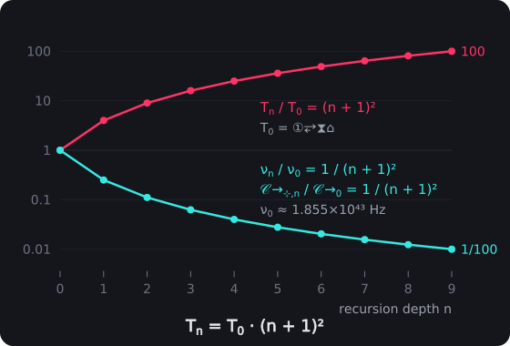
Temporal Drag Across Recursion Depth. The Recursive Pulse Cycle Time Tₙ = T₀ · (n + 1)² grows a hundredfold by depth n = 9, while the pulse frequency νₙ = ν₀/(n + 1)² and the effective light speed 𝒞→⊹,n = 𝒞→₀/(n + 1)² fall by the same factor, from T₀ = ①⥂⧗⌂ and ν₀ ≈ 1.855 × 10⁴³ Hz. The effective speed is an average through structure; the step speed stays 𝒞→. The tick T₀ itself is the same at every depth; Tₙ counts (n + 1)² of them.
7.4 Testable Predictions
- Quadratic Cycle Counts: A depth-n cycle spans T_n = T_0 × (n + 1)² ticks of the fixed Planck interval in layered recursive systems; the tick itself does not change inside a universe, so the signature is the (n + 1)² ratio between cycle lengths at different depths, not a slower local clock, measurable by timing cycles across structural depths.
- Discrete Temporal Granularity: Characteristic time scales T_n = T_0 × (n + 1)², whole multiples of the fixed Planck interval, observable through precision timing in quantum systems.
- Harmonic Clock Modulation: Recursive cycle frequencies following ν_n = ν_0/(n + 1)², each depth-n cycle counting P(n) = (n+1)² of the same tick (a clock's own tick does not change with depth), detectable via frequency stability analysis as (n+1)² frequency ratios between depths.
- Information Processing Delays: Scaling Δt⊶,n = T_0 × L_n/L⥣ in quantum computational systems, quantifiable through computational benchmarking.
- Enhanced Redshift: A depth-n cycle spans (n + 1)² ticks of the fixed interval, so its signal, read against a depth-0 cycle, shows the cycle-count ratio z⇜(n) = (n + 1)² - 1; the local clock does not slow, observable in gravitational wave timing.
- Causal Disconnection: Between temporal regimes when Δtℹ > T_n in ultra-deep recursive layers, testable through information transmission experiments.