Chapter 9 · Section 9
The Ignition Moment — When Potential Becomes Reality
The Computational Physical Nova (Big Bang)
What triggers the transition from timeless computational potential to explosive emergence of spacetime itself — the moment when recursive processing reaches critical threshold and ignites dimensional reality? Binary Pulse Theory fundamentally reconceptualizes cosmic emergence as Computational Phase Transition (G) driven by Recursive Amplification rather than spontaneous quantum fluctuation, where Universe's birth occurs when Prime Pulse substrate achieves Critical Recursive Density through Cascading Feedback Loops — the computational equivalent of the Big Bang.
This proposal describes a mechanism triggering cosmic genesis from computational potential through deterministic Ignition Loop rather than mysterious initial conditions. Building upon the inevitable emergence principle from Part 9.4, where null states cannot persist indefinitely and must resolve into structured existence, Ignition Process represents the moment when computational potential transforms into dimensional reality through recursive mechanisms.
Connecting to phase alignment dynamics from Part 9.5, where phase relationships can accelerate or delay recursive processing, and π-defined harmonic structure from Part 9.8, where Resonance Conditions (G) follow same geometric principles governing binary transitions, Ignition Loop describes how Phase-Synchronized Recursion creates explosive amplification culminating in dimensional emergence.
Guth's inflationary paradigm (Guth, 1981)³⁸ and Penrose's cyclic cosmology (Penrose, 2010)⁹ describe beginnings driven by rapid transitions; in BPT, Information Conservation I⊚ = I▱ + Iℜ encounters Critical Overflow Conditions through Recursive Density Accumulation. The resulting cascade represents the computational equivalent of Big Bang — the Physical Nova triggering transition from pure potential to physical reality through deterministic rather than random processes.
The essential insight recognizes that ignition defines Absolute Beginning of Temporal Structure (G) within emergent domain, transforming Pre-Pulse Field geometry from Part 9.7 into structured spacetime supporting all subsequent evolution.
Pre-Ignition Dynamics and Loop Formation
The Pre-Ignition Dynamics and Loop Formation stage defines the unstable balance preceding recursive amplification, where random fluctuations remain suspended between dissipation and ignition. In this regime, proto-nova probabilities and recursive stability thresholds determine whether isolated concentrations of energy collapse back into noise or accumulate into stable loops capable of fueling recursive processing.
Before recursive amplification, the substrate exhibits Equilibrium Conditions characterized by Fluctuation Statistics. Mean Energy Condition (G) ⟨E⌇⟩ = 0 [J] and variance Var(E⌇) = σ²▱ [J²] characterize random substrate variations where σ²▱ represents Fluctuation Amplitude in Pre-Pulse Field from Part 9.7.
Proto-Nova Formation Probability determines isolated energy concentration likelihood:
Proto-Nova Formation Probability G
P(◁✺) = exp(-E⨶/(k_B T▱)) [∅]
Where:
- P(◁✺) [∅] - proto-nova formation probability
- exp [∅] - exponential function
- E⨶ [𝕄·𝕃²·𝕋⁻²] - energy threshold
- k_B [𝕄·𝕃²·𝕋⁻²·Θ⁻¹] - Boltzmann constant
- T▱ [Θ] - substrate temperature
➢ Isolated Energy Concentrations remain transient because they lack Recursive Feedback necessary for Self-Amplification, consistent with null state instability from Part 9.4 where structures must emerge through recursive processing.
Recursive Stability Criterion connects to phase alignment from Part 9.5.
Recursive Stability Criterion G
R⫷(n) = Σ_{i=1}^n ΔE_i × f≍(i) ≥ R⨶ [J]
Where:
- R⫷(n) [𝕄·𝕃²·𝕋⁻²] - recursive accumulation function
- Σ [∅] - summation operator
- i [∅] - cycle index
- 1 [∅] - summation lower limit
- n [∅] - total number of cycles
- ΔE_i [𝕄·𝕃²·𝕋⁻²] - energy retained in ith cycle
- f≍(i) [∅] - correlation function between cycles enhanced by phase alignment
- R⨶ [𝕄·𝕃²·𝕋⁻²] - minimum threshold for loop stability
Dimensional analysis:
Where (from the book): 1 [∅], Σ [∅], i [∅], n [∅], ΔE_i [𝕄·𝕃²·𝕋⁻²], f≍(i) [∅], R⨶ [𝕄·𝕃²·𝕋⁻²]
Read dimensionally: R⫷(n) = ΔE_i × f≍(i) ≥ R⨶
[𝕄·𝕃²·𝕋⁻²]
[𝕄·𝕃²·𝕋⁻²] × [∅] ≥ [𝕄·𝕃²·𝕋⁻²] = [𝕄·𝕃²·𝕋⁻²] ≥ [𝕄·𝕃²·𝕋⁻²]
[𝕄·𝕃²·𝕋⁻²] = [𝕄·𝕃²·𝕋⁻²] ≥ [𝕄·𝕃²·𝕋⁻²] ✓ Valid PulseCore Verified ✓
➢ Phase alignment enhancement from Part 9.5 accelerates recursive accumulation toward critical ignition threshold through correlation-enhanced energy retention that establishes loop stability requirements for recursive processing.
The Memory Accumulation Equation characterizes information persistence:
Memory Accumulation Equation G
S_n = S_{n-1} × α𝓜 + I▷ × β⧱ [J/K]
Where:
- S_n [𝕄·𝕃²·𝕋⁻²·Θ⁻¹] - system memory at cycle n
- S_{n-1} [𝕄·𝕃²·𝕋⁻²·Θ⁻¹] - system memory at cycle n-1
- α𝓜 [∅] - memory persistence coefficient
- I▷ [𝕄·𝕃²·𝕋⁻²·Θ⁻¹] - new information input
- β⧱ [∅] - coupling strength enhanced by Phase Coupling Equation
- n [∅] - current cycle index
- C(φ₁, φ₂) [∅] - Phase Coupling Equation
- α [∅] - cosine coupling coefficient
- cos [∅] - cosine function
- Δφ [∅] - phase difference
- β [∅] - sine coupling coefficient
- sin [∅] - sine function
- φ₁ [∅] - phase one
- φ₂ [∅] - phase two
Dimensional analysis:
Where (from the book): S_n [𝕄·𝕃²·𝕋⁻²·Θ⁻¹], S_{n-1} [𝕄·𝕃²·𝕋⁻²·Θ⁻¹], α𝓜 [∅], I▷ [𝕄·𝕃²·𝕋⁻²·Θ⁻¹], β⧱ [∅], n [∅], C(φ₁, [∅], α [∅], cos [∅], β [∅], sin [∅]
[𝕄·𝕃²·𝕋⁻²·Θ⁻¹]
[𝕄·𝕃²·𝕋⁻²·Θ⁻¹] × [∅] + [𝕄·𝕃²·𝕋⁻²·Θ⁻¹] × [∅] = [𝕄·𝕃²·𝕋⁻²·Θ⁻¹] + [𝕄·𝕃²·𝕋⁻²·Θ⁻¹] × [∅] = [𝕄·𝕃²·𝕋⁻²·Θ⁻¹] + [𝕄·𝕃²·𝕋⁻²·Θ⁻¹] = [𝕄·𝕃²·𝕋⁻²·Θ⁻¹]
[𝕄·𝕃²·𝕋⁻²·Θ⁻¹] = [𝕄·𝕃²·𝕋⁻²·Θ⁻¹] ✓ Valid PulseCore Verified ✓
➢ Phase coupling enhancement drives memory persistence and information integration through retention and coupling mechanisms that establish system memory evolution dynamics.
Together, the ignition probability, stability criterion, and memory accumulation equation demonstrate how transient fluctuations cross into sustained recursion through correlation-enhanced feedback and information retention. Pre-ignition thus marks the decisive threshold where random noise either decays or self-organizes into enduring loops, laying the foundation for ignition, recursion, and emergent structure. In this light, loop formation is not accidental but the necessary precondition for computation itself—where stability arises from alignment, memory, and recursive feedback woven into the substrate.
Critical Resonance and Harmonic Amplification
The Critical Resonance and Harmonic Amplification (G) stage describes how recursive oscillations surpass equilibrium, with π-derived harmonics and phase alignment driving exponential growth. Here, resonance conditions and amplification dynamics determine whether fluctuations remain bounded or ignite into full recursive cascades. Exponential Growth Dynamics follow π-derived resonance from Part 9.8.
Exponential Growth Dynamics G
A(t) = A₀ × exp(γt) × sin(ωt + φ) [∅]
Where:
- A(t) [∅] - amplitude of recursive oscillation
- A₀ [∅] - initial amplitude
- exp [∅] - exponential function
- γ [𝕋⁻¹] - exponential growth rate
- t [𝕋] - time variable
- sin [∅] - sine function
- ω [𝕋⁻¹] - fundamental recursion frequency (π/τ⥂ following π-Harmonic Structure)
- φ [∅] - phase offset enabling Alignment Acceleration from Part 9.5
- π [∅] - mathematical constant pi
- τ⥂ [𝕋] - Pulse period
➢ π-derived resonance from Part 9.8 combined with phase alignment from Part 9.5 creates exponential amplification toward ignition through oscillatory growth patterns that establish amplification dynamics toward critical thresholds.
The Resonance Condition extends π-geometry from Part 9.8.
Resonance Condition
ω◌ = n × ω⥂ × (1 ± Δω) [rad/s]
Where:
- ω◌ [𝕋⁻¹] - driving frequency
- n [∅] - harmonic number
- ω⥂ [𝕋⁻¹] - natural frequency (π/τ⥂)
- 1 [∅] - unity constant
- Δω [∅] - detuning parameter
- π [∅] - mathematical constant pi
- τ⥂ [𝕋] - Pulse period
➢ When driving frequency matches natural harmonics following the same π-derived resonance conditions from Emergence Arc, Constructive Interference creates explosive amplification accelerated through phase alignment mechanisms.
The Physical Nova Ignition Threshold accumulates recursive processing.
Physical Nova Ignition Threshold G
T⫷ = ∫₀^t P(τ) × R⫷(τ) dτ [𝕄·𝕃²·𝕋⁻²]
Where:
- T⫷ [𝕄·𝕃²·𝕋⁻²] - accumulated threshold parameter
- ∫ [∅] - integration operator
- ₀ [𝕋] - integration lower limit
- t [𝕋] - integration upper limit
- P(τ) [𝕋⁻¹] - processing rate
- R⫷(τ) [𝕄·𝕃²·𝕋⁻²] - recursive strength
- τ [𝕋] - integration variable
Dimensional analysis:
Where (from the book): T⫷ [𝕄·𝕃²·𝕋⁻²], ₀ [𝕋], t [𝕋], P(τ) [𝕋⁻¹], R⫷(τ) [𝕄·𝕃²·𝕋⁻²], τ [𝕋]
Read dimensionally: T⫷ = P(τ) × R⫷(τ) × (τ)
[𝕄·𝕃²·𝕋⁻²]
[𝕋⁻¹] × [𝕄·𝕃²·𝕋⁻²] × ([𝕋]) = [𝕄·𝕃²·𝕋⁻³] × [𝕋] = [𝕄·𝕃²·𝕋⁻²]
[𝕄·𝕃²·𝕋⁻²] = [𝕄·𝕃²·𝕋⁻²] ✓ Valid PulseCore Verified ✓
➢ Integral accumulation of recursive processing over time. Ignition Condition defines transition moment: If T⫷ ≥ T⨶, then ✹ = TRUE — threshold represents the moment when recursive processing transitions from potential to dimensional reality, establishing the Absolute Beginning of Temporal Structure within the emergent domain.
Together, the exponential growth law, resonance condition, and ignition threshold reveal how oscillatory feedback evolves into runaway amplification. Once harmonic resonance locks to π-based geometry, constructive interference accelerates recursive accumulation until the ignition boundary is crossed. In this light, critical resonance is not just a mathematical artifact but the decisive bridge where aligned oscillations pass from fragile fluctuation into irreversible amplification, marking the true birth of dimensional structure.
Dimensional Emergence Cascade and Timeline
The Dimensional Emergence Cascade and Timeline describes how recursive density fields evolve through self-organized criticality, driving the universe from equilibrium fluctuations into structured dimensional phases. Governed by diffusion, nonlinear growth, decay, and stochastic perturbations, this cascade represents the mathematical framework by which spontaneous order arises from critical instability. Self-Organized Criticality Dynamics govern the emergence cascade.
Self-Organized Criticality Dynamics G
∂ρℜ/∂t = D ∇² ρℜ + f(ρℜ) - γ ρℜ + η(x,t) [kg/(m³·s)]
Where:
- ∂ρℜ/∂t [𝕄·𝕃⁻³·𝕋⁻¹] - time derivative of recursive density field
- ρℜ [𝕄·𝕃⁻³] - recursive density field
- D [𝕃²·𝕋⁻¹] - diffusion coefficient
- ∇² [𝕃⁻²] - Laplacian operator
- f(ρℜ) [𝕄·𝕃⁻³·𝕋⁻¹] - nonlinear growth function
- γ [𝕋⁻¹] - decay rate
- η(x,t) [𝕄·𝕃⁻³·𝕋⁻¹] - noise term
- x [𝕃] - spatial position
- t [𝕋] - time variable
➢ Sornette's self-organized criticality (Sornette, 2006)³⁹ demonstrates how complex systems spontaneously evolve into critical states, poised for phase transitions. Brandenberger's cosmic inflation (Brandenberger, 2017)⁴⁰ shows comparable Folding Effects in string-theoretic brane scenarios where localized tension in higher-dimensional membranes restructures geometry prefiguring emergent spacetime metrics. The Critical Growth Function exhibits a characteristic S-Curve.
Critical Growth Function G
f(ρℜ) = α ρℜ - β ρℜ³ + δ ρℜ⁵ [kg/(m³·s)]
Where:
- f(ρℜ) [𝕄·𝕃⁻³·𝕋⁻¹] - critical growth function
- α [𝕋⁻¹] - linear growth coefficient
- ρℜ [𝕄·𝕃⁻³] - recursive density field
- β [𝕄⁻²·𝕃⁶·𝕋⁻¹] - cubic suppression coefficient
- δ [𝕄⁻⁴·𝕃¹²·𝕋⁻¹] - quintic enhancement coefficient
➢ Polynomial exhibits characteristic S-curve of phase transitions with Unstable Intermediate States leading to dimensional emergence through nonlinear growth dynamics that establish critical transition behavior in substrate architectures.
Taken together, the self-organized criticality dynamics and nonlinear growth functions reveal how recursive density fields cross thresholds into unstable intermediate states, producing the characteristic S-curve of emergent transitions. Each phase of the cascade marks a shift where random fluctuations give way to organized structure, guided by tension, resonance, and recursive feedback. In this light, the dimensional emergence cascade is not merely a sequence of transitions but the universal timeline through which spacetime itself unfolds, charting the irreversible march from chaos to coherent dimensional order.
Emergence Timeline and Information Processing
The Emergence Timeline and Information Processing outlines the structured progression by which random fluctuations in the substrate evolve into ordered dimensional reality. Beginning with undefined pre-ignition states, the timeline traces recursive loop formation, exponential amplification, critical thresholds, and finally the ignition of dimensional emergence, situating spacetime expansion within a recursive cycle framework. Information-theoretic analysis complements this sequence, quantifying inevitability by decomposing the conserved total information into substrate and recursive components, with the correlation information carried inside the recursive part.
Emergence Timeline Sequence G
Phase | Duration (the data's count, no universe time) | Recursive Cycles (Zinf cycles) | Key Events |
|---|---|---|---|
Pre-ignition | Undefined | 0 | Random fluctuations only |
~10³ ①⥂⧗⌂ | 1-10² | Recursive patterns emerge | |
Amplification (G) | ~10² ①⥂⧗⌂ | 10²-10⁴ | Exponential growth begins |
~10¹ ①⥂⧗⌂ | 10⁴-10⁶ | Threshold proximity | |
~1 ①⥂⧗⌂ | 10⁶+ | Dimensional emergence | |
Ongoing | Continuous | Spacetime evolution |
Where:
- ①⥂⧗⌂ [𝕋] - Local Pulse Tempo (Planck time), here a step of the data's count: everything before the Physical Nova takes no universe time (the universe's life counts from the Physical Nova)
- 10³ [∅] - duration coefficient for Loop Formation
- 10² [∅] - upper cycle limit for Loop Formation / duration coefficient for Amplification
- 10⁴ [∅] - upper cycle limit for Amplification / upper cycle limit for Critical Approach
- 10¹ [∅] - duration coefficient for Critical Approach
- 10⁶ [∅] - cycle threshold for Nova Ignition, counted in Zinf cycles ℨ: one Tempo holds s ≈ 2.361 × 10⁶² of them, so 10⁶+ cycles fit within ~1 ①⥂⧗⌂
- 1 [∅] - duration coefficient for Nova Ignition
➢ Emergence Timeline Sequence establishes fundamental temporal progression from random fluctuations through recursive pattern formation to dimensional emergence and spacetime evolution, demonstrating how emergence phases progress systematically through increasing recursive cycle complexity toward dimensional manifestation.
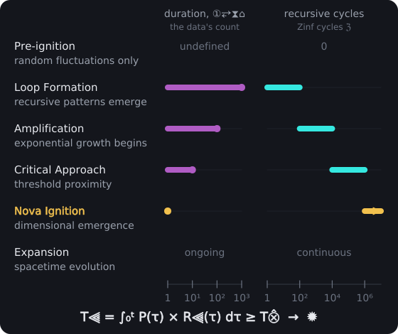
The Road to Ignition. From loop formation to nova ignition, each phase is about ten times shorter in Planck-time steps of the data's count (no universe time passes before the Physical Nova) while its recursive cycles grow a hundredfold. Ignition comes when the accumulated threshold T⫷ reaches T⨶, and dimensional emergence begins.
Information-Theoretic Analysis quantifies emergence inevitability.
Information-Theoretic Analysis G
I⊚ = I▱ + Iℜ [1ᵇ]
Where:
- I⊚ [1ᵇ] - total information content
- I▱ [1ᵇ] - substrate information component
- Iℜ [1ᵇ] - recursive information component
- I≍ [1ᵇ] - correlation (mutual) information, the part of Iℜ held in correlations; it is counted inside Iℜ, not added to it
Dimensional analysis:
Where (from the book): I⊚ [1ᵇ]
[1ᵇ]
[1ᵇ] + [1ᵇ] = [1ᵇ]
[1ᵇ] = [1ᵇ] ✓ Valid PulseCore Verified ✓
➢ Information-theoretic analysis quantifies emergence inevitability through total information decomposition, I⊚ = I▱ + Iℜ with the correlation information I≍ inside Iℜ, that demonstrates how substrate and recursive components establish information-driven emergence dynamics.
Mutual Information Growth G
dI≍/dt = (1/①⥂⧗⌂) × Σ_{i,j} R_{ij} × log₂(R_{ij}/(R_i × R_j)) · ℨᵇ [𝕋⁻¹·1ᵇ]
Where:
- dI≍/dt [𝕋⁻¹·1ᵇ] - mutual information growth rate, in Zinf bits per Tempo
- I≍ [1ᵇ] - mutual information, in Zinf bits
- Σ [∅] - summation operator
- i [∅] - first correlation index
- j [∅] - second correlation index
- R_{ij} [∅] - joint correlation frequencies, normalized
- log₂ [∅] - logarithm base 2 function
- R_i [∅] - marginal correlations for index i
- R_j [∅] - marginal correlations for index j
- t [𝕋] - time variable
- ①⥂⧗⌂ [𝕋] - one Pulse Tempo: the sum is the mutual information one Tempo adds
Dimensional analysis:
Where (from the book): dI≍/dt [𝕋⁻¹·1ᵇ], Σ [∅], i [∅], j [∅], R_{ij} [∅], log₂ [∅], R_i [∅], R_j [∅], t [𝕋]
Read dimensionally: dI≍/dt = (1/①⥂⧗⌂) × R_{ij} × log₂(R_{ij}/(R_i × R_j)) · ℨᵇ
[𝕋⁻¹·1ᵇ]
([∅] ÷ [𝕋]) × [∅] × [∅]([∅] ÷ ([∅] × [∅])) × [1ᵇ] = [𝕋⁻¹] × [∅] × [∅]([∅] ÷ ([∅] × [∅])) × [1ᵇ] = [𝕋⁻¹] × [∅]([∅] ÷ ([∅] × [∅])) × [1ᵇ] = [𝕋⁻¹] × [∅]([∅] ÷ [∅]) × [1ᵇ] = [𝕋⁻¹] × [∅]([∅]) × [1ᵇ] = [𝕋⁻¹] × [∅] × [1ᵇ] = [𝕋⁻¹] × [1ᵇ] = [𝕋⁻¹·1ᵇ]
[𝕋⁻¹·1ᵇ] = [𝕋⁻¹·1ᵇ] ✓ Valid PulseCore Verified ✓
➢ Describes how Recursive Correlations increase system-wide information content, driving emergence through Information Conservation principles. Penrose's conformal cyclic cosmology (Penrose, 2010)⁹ and Steinhardt and Turok's cyclic Universe model (Steinhardt & Turok, 2007) demonstrate conceptual similarities with continuous cycle of recursive processing and dimensional emergence.
Together, the Emergence Timeline Sequence and information-theoretic framework reveal that dimensional manifestation is not a contingent accident but the natural outcome of recursive information growth. Each phase in the timeline—from fluctuations to ignition—marks an inevitable step in the upward sweep of correlation and recursion, where increasing density of information drives structure into being. Mutual information growth, though dimensionally challenging, captures the principle that correlations themselves serve as engines of emergence, amplifying systemic order from noise. In this light, the ignition of spacetime is best understood as the critical threshold of an information-driven cascade, where recursive cycles, once self-sustaining, transform potential into the unfolding continuum of reality.
Quantum Field Integration and Cosmological Parameters
Before equations can formalize the universe’s beginning, the substrate itself must decide how fields and geometry interlock. At this frontier, quantum fields are not isolated variables but recursive engines, folding fluctuations into order until instability tips into expansion. What emerges is less a static equation and more a negotiation between recursion, vacuum instability, and the birth of spacetime parameters themselves. Effective Field Equations incorporate recursive dynamics.
Effective Field Equations G
□φ + m²φ + λ φ³ + g × R_op[φ] = 0 [kg/(m·s²)]
Where:
- □ [𝕋⁻²] - d'Alembertian operator (∂²/∂t² - 𝒞→²∇²)
- φ [∅] - field variable
- m [𝕄·𝕋⁻¹] - effective mass
- λ [𝕄⁻¹·𝕃³·𝕋⁻²] - self-interaction coupling
- g [𝕋⁻³] - Recursive Coupling Constant
- R_op[φ] [𝕄·𝕃·𝕋⁻¹] - recursive operator implementing evolution
- ∂²/∂t² [𝕋⁻²] - second time derivative
- 𝒞→ [𝕃·𝕋⁻¹] - speed of light
- ∇² [𝕃⁻²] - Laplacian operator
- 0 [𝕄·𝕃⁻¹·𝕋⁻²] - null value
➢ Recursive coupling modifies standard field equations, showing how computational dynamics drive field evolution through recursive operator implementation that establishes modified field dynamics incorporating computational processes.
Vacuum Instability Condition G
∂²V⊹/∂φ²|_{φ=0} < 0 [𝕄·𝕃²·𝕋⁻²]
Where:
- ∂²V⊹/∂φ² [𝕄·𝕃²·𝕋⁻²] - second derivative of effective potential with respect to field (an energy, as V⊹ is and φ is dimensionless)
- V⊹ [𝕄·𝕃²·𝕋⁻²] - effective potential
- φ [∅] - field variable
- 0 [∅] - evaluation point (φ = 0)
Dimensional analysis:
Where (from the book): 0 [∅], ∂²V⊹/∂φ² [𝕄·𝕃²·𝕋⁻²], V⊹ [𝕄·𝕃²·𝕋⁻²], φ [∅]
Read dimensionally: ∂²V⊹/∂φ² < 0
[𝕄·𝕃²·𝕋⁻²] < [∅] ✓ Valid PulseCore Verified ✓
➢ Recursive substrate becomes unstable to small perturbations when Vacuum Instability Condition is met, triggering ignition. Linde's inflationary cosmology (Linde, 2008)⁴¹ describes rapid, exponential expansion following a comparable instability, analogous to Inflationary Epoch where scalar field drives explosive space expansion.
Altogether, the recursive formulation of effective field equations and the vacuum instability condition reveal that cosmological unfolding is inseparable from computational recursion. Once instability is triggered, recursive operators magnify perturbations into exponential growth, echoing inflationary cosmology while grounding expansion in information-driven recursion. In this light, the origin of spacetime is seen not only as a scalar field phenomenon but as the inevitable consequence of recursive field dynamics—where instability, amplification, and inflation emerge as stages of one unified process.
Cosmological Parameter Relationships
Cosmic parameters are not merely observational constants but recursive markers, encoding how expansion, density, and recursion interlock. The Hubble constant and critical density emerge as dual expressions of the same substrate law — one governing the rhythm of expansion, the other the balance point of matter and geometry. In Binary Pulse Theory, these parameters become diagnostic signals of recursion itself, revealing how local measurement reflects the deeper recursive structure of the cosmos. The Hubble Constant Connection links expansion to recursion.
Hubble Constant Connection G
H₀ = (γℜ × 𝒞→) / L◎ [𝕋⁻¹]
Where:
Dimensional analysis:
Where (from the book): γℜ [∅], L◎ [𝕃]
[𝕋⁻¹]
([∅] × [𝕃·𝕋⁻¹]) ÷ [𝕃] = [𝕃·𝕋⁻¹] ÷ [𝕃] = [𝕋⁻¹]
[𝕋⁻¹] = [𝕋⁻¹] ✓ Valid PulseCore Verified ✓
➢ Cosmic expansion rate directly reflects recursive amplification parameters through the relationship between recursive rate and horizon scale that establishes expansion dynamics in substrate architectures.
Critical Density Relation G
ρ⨶ = (3H₀²) / (8πG) × Fℜ [𝕄·𝕃⁻³]
Where:
- ρ⨶ [𝕄·𝕃⁻³] - critical cosmic density
- 3 [∅] - numerical coefficient
- H₀ [𝕋⁻¹] - Hubble constant
- 8π [∅] - geometric factor
- G [𝕄⁻¹·𝕃³·𝕋⁻²] - gravitational constant
- Fℜ [∅] - recursive amplification factor embedded in cosmic expansion
- 8 [∅] - coefficient
- π [∅] - mathematical constant pi
➢ Critical cosmic density modified by recursive coupling embedded in expansion dynamics following the same principles governing emergence from computational substrate that establishes density modification through recursive amplification factors.
Thus, cosmological parameters like the Hubble constant and critical density cease to be arbitrary values tuned by chance. They are mathematical shadows of recursive amplification, where expansion rate and density balance encode the same universal negotiation between computation and geometry. In this light, the constants of cosmology become recursion’s signature written into spacetime — measurable numbers that whisper the recursive law of reality itself.
9.9 Testable Predictions
- Cosmic Microwave Background Non-Gaussian Statistics: From Recursive Correlations following dI≍/dt = (1/①⥂⧗⌂) × Σ_{i,j} R_{ij} × log₂(R_{ij}/(R_i × R_j)) · ℨᵇ information growth detectable with sensitivity better than 10⁻⁶, observable through higher-order statistical analysis of temperature and polarization maps revealing systematic deviations from Gaussian random field predictions.
- Primordial Gravitational Wave Frequency Spectrum: Exhibiting π-Harmonic Resonance Patterns from ω◌ = n × ω⥂ × (1 ± Δω) conditions detectable by future space-based observatories, identifiable through spectral analysis revealing characteristic π-spaced frequency peaks in the primordial gravitational wave background.
- Large-Scale Structure Fractal Patterns: Reflecting Recursive Density Evolution ∂ρℜ/∂t = D ∇² ρℜ + f(ρℜ) - γ ρℜ + η(x,t) cascade dynamics, measurable through multi-scale correlation analysis of galaxy distribution patterns showing self-similar hierarchical structure formation.
- Hubble Constant Relationship: H₀ = (γℜ × 𝒞→) / L◎ connecting expansion rate to Recursive Amplification Parameters with precision better than 1%, testable through independent measurements of cosmic expansion rate showing systematic correlation with recursive parameter estimates.
- Critical Density Modifications: ρ⨶ = (3H₀²) / (8πG) × Fℜ from recursive coupling embedded in cosmic expansion, quantifiable through precision cosmological parameter estimation revealing systematic deviations from standard critical density predictions.
- Vacuum Instability Signatures: In quantum field experiments exhibiting ∂²V⊹/∂φ²|_{φ=0} < 0 threshold behavior, observable through precision measurements of vacuum state stability showing characteristic instability onset at critical field strength thresholds.
These predictions outline a framework for understanding cosmic genesis as computational ignition — a proposed mechanism triggering transition from timeless potential to explosive dimensional reality through deterministic Ignition Loop dynamics rather than mysterious initial conditions.
Chapter Review: The Computational Universe
Chapter 9 has presented Binary Pulse Theory as an information-first framework that reframes reality as an active, self-modifying computational process. Beginning with the reading of dark matter as Computational Resolution Failures rather than exotic particles, we traced how the Universe's structure emerges from incomplete Pulse processing within discretized binary substrate — a computational account of one of physics' greatest open questions.
Discoveries Across All Scales
The Foundational Architecture progression through Density-Dependent Temporal Resolution proposed that temporal resolution varies with collapse density, inverting the usual picture of temporal fundamentals. Instead of Planck time being a universal constant, it emerges from density-encoded mechanisms that connect each universe's collapse conditions to its computational capacity — so different universes run at different resolutions, while within any one universe the Planck time stays fixed.
Parametric Inheritance proposed that physical constants evolve like cosmic DNA across Universe generations with systematic variations that address the fine-tuning problem through evolutionary cosmology rather than anthropic selection. The Master Evolution Equation governs this cosmic genealogy, creating deterministic yet diverse Recursive Cosmological Tree structures.
BPT's response to "why something rather than nothing" emerged through arguing that existence is computationally inevitable. The Null Potential Integral provides a mathematical argument that emergence becomes inevitable through computational cycles, while Universal Emergence Mechanisms operate across all recursive layers from quantum vacuum to cosmological scales — arguing for existence as logical necessity rather than cosmic accident.
Advanced Capabilities and Technologies
Phase Modulation Navigation (G) proposed movement through computational substrate manipulation, with effective displacement rates beyond 𝒞→ drawn from substrate geometry, while the vehicle never exceeds 𝒞→ locally and no message outruns light. The Phase Projection Operator enables predictive trajectory planning through substrate manipulation, opening possibilities for advanced propulsion systems based on phase dynamics rather than conventional acceleration.
Symmetry Breaking (G) dynamics proposed that perfect symmetry cannot persist when recursive computation overflows system capacity. The Overflow Condition offers an account of why the Universe exhibits structure through computational necessity rather than arbitrary initial conditions, while Force Genesis emerges through recursive asymmetries modifying fundamental interactions.
Information Foundation and Geometric Principles
The Pre-Pulse Field proposed information as eternal — existing in a timeless field before temporal evolution begins, addressing information paradoxes by reading the deepest foundation as pure computational possibility preceding all structure. The Information Potential Functional governs evolution prior to temporal structure, while Data Convergence Formation seeds all subsequent dimensional emergence.
The geometric significance of π as the first emergent mathematical constant from computational necessity offers an account of why it appears throughout physics as the intrinsic constant of reality's computational substrate. The Emergence Arc Function demonstrates how π defines optimal trajectories through Binary State Space, establishing the geometric foundation of binary computation.
Finally, the Ignition Loop proposed a mechanism triggering cosmic genesis from computational potential through deterministic phase transitions rather than mysterious initial conditions. The Physical Nova represents the computational equivalent of the Big Bang, establishing the Absolute Beginning of Temporal Structure through Recursive Amplification reaching a critical threshold.
Testable Predictions and Empirical Validation
Throughout all parts, Binary Pulse Theory shows coherence across scales from quantum vacuum fluctuations to cosmic expansion. The framework provides specific testable predictions spanning:
- Dark Matter Signatures: Resolution-dependent profiles deviating from NFW models in high-resolution regions, detectable through gravitational lensing analysis
- Frequency Deviations: Measurable differences Δf = f⌾ - f⊢_GR between observed frequencies and general relativity predictions
- Temporal Resolution Effects: CMB temperature anisotropies exhibiting density-dependent amplitude variations following f(ρ⦰) scaling
- Constant Evolution: Fine structure constant variations Δα/α ≈ 10⁻⁶ correlated with density-dependent temporal resolution
- Phase Navigation: Quantum entanglement phase timing exhibiting controlled substrate manipulation effects
- Symmetry Breaking: CMB non-Gaussian features from recursive defect networks with sensitivity better than 10⁻⁶
- Information Foundations: Vacuum Casimir effect modifications from pre-causal boundary conditions
- π-Geometric Effects: Atomic transition phase relationships exhibiting π-periodic patterns with precision better than 10⁻⁹
- Genesis Signatures: Primordial gravitational wave frequency spectrum exhibiting π-harmonic resonance patterns
Impact on Physics and Philosophy
Most significantly, Binary Pulse Theory proposes information as the primary substrate from which matter, energy, spacetime, and physical laws emerge through recursive computational processes. This information-first Universe positions consciousness and awareness as natural developments within a computational substrate, suggesting that recursive information processing capabilities enabling technological singularity represent continuation of the same computational principles underlying physical reality itself.
The framework establishes a foundation for understanding how Information Recursion shapes evolution of universal laws while providing pathways for advanced navigation through spacetime's computational substrate. Computational Cosmology emerges as a new field studying Universe evolution through information processing dynamics.
Future Directions and Research Opportunities
The framework opens immediate research opportunities in:
- Experimental Validation: Frequency Deviation Tests providing concrete pathways for empirical validation through precision measurements
- Advanced Propulsion: Phase Navigation Principles suggesting practical applications for future space exploration technologies
- Computational Physics: Information-theoretic approaches to fundamental physical phenomena
- ✧ Studies: Understanding awareness emergence through computational substrate dynamics
- Cosmological Engineering: Practical applications of temporal resolution and parametric inheritance principles
The Deepest Implication: Reality as Living Computation
In Binary Pulse Theory, reality itself is living computation — an active, self-modifying information processing system where consciousness, physics, and cosmic evolution represent different manifestations of the same underlying computational substrate architecture. This framework provides both testable predictions for immediate experimental validation and insights into the nature of existence as inevitable computational emergence from logical necessity.
The Arc of Emergence traced throughout Chapter 9 points toward a Universe where information, computation, and consciousness are the fundamental drivers of cosmic evolution, enabling the emergence of ever-greater complexity and awareness for as long as the Universe runs. That run is finite: every bit returns through a singularity on its loop home, and a universe ends when all its bits have returned; then a new UniSphere bifurcates in each of its wells, one level deeper (Chapter 3), and the arc begins again. Binary Pulse Theory is offered as a framework for understanding reality's computational foundations.